Many Google Sheets functions are available to make using Excel (or Google Sheets) easier and more efficient. In this article, we will discuss one of the important functions: the SUM function. The SUM function in Excel (or Google Sheets) lies in its fundamental role in performing basic arithmetic operations and facilitating data analysis, such as basic calculation or data analysis.
In this article, you will learn about the SUM function, how to use it, and its differences from the SUMIF function. At the end, you will find a section with commonly asked questions.
What is the SUM function in Google Sheets?
The SUM function in Google Sheets is employed to calculate the total of a sequence of numbers or individual values. It is widely utilized for performing fundamental arithmetic computations within spreadsheet data, such as adding up a set of numbers or specific values.
When to use the SUM function?
The SUM function in Google Sheets is extremely useful in a variety of scenarios where you need to perform arithmetic operations on a series of numbers. Here are some common situations when you might use the SUM function:
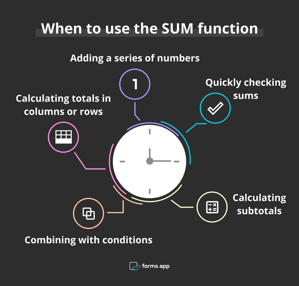
Right times to use the SUM function
⏰Adding a series of numbers
⏰Calculating totals in columns or rows
⏰Combining with conditions
⏰Calculating subtotals
⏰Quickly checking sums
💡You can also check the article about the XLOOKUP function.
How to use the SUM Function?
Using the SUM function in Google Sheets is straightforward and allows you to quickly calculate the total of a range of numbers or specific values. If you are wondering how, here are steps to learn how to use the SUM function in detail:
1. Open Google Sheets

Open your Sheet
Go to Google Sheets and open the spreadsheet where you want to use the SUM function.
2. Select a cell

Click a blank cell
Click on the cell where you want the result of the SUM function to appear.
3. Type the function
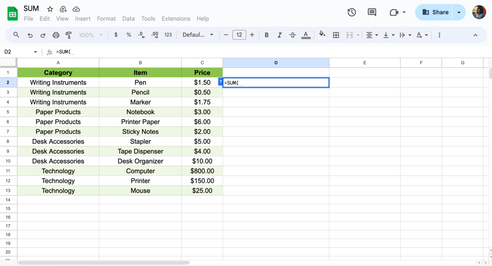
Start typing the function
In the selected cell, start typing =SUM( to begin the SUM function.
4. Specify the range of numbers
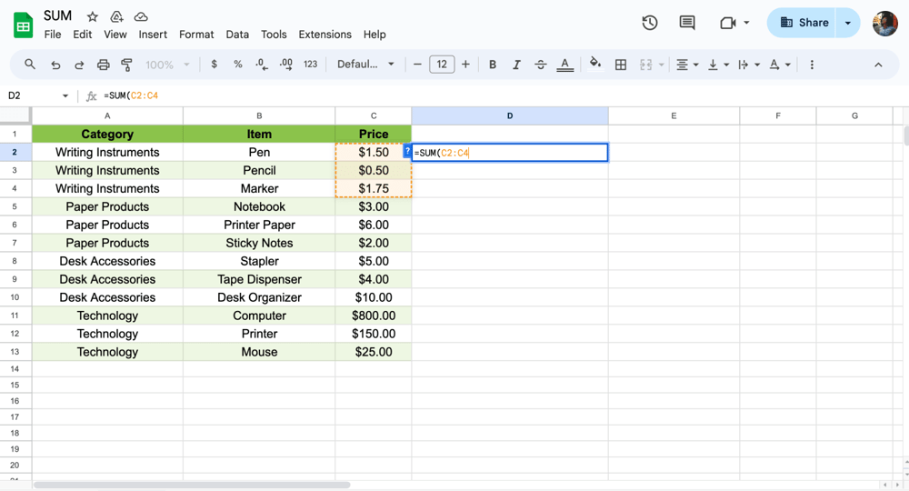
Choose the correct cells
- Individual Cells: You can directly reference individual cells by typing their cell references separated by commas. For example: =SUM(A1, B1, C1)
- Range of Cells: Specify a range of cells by typing the starting cell reference followed by a colon (:) and then the ending cell reference. For example: =SUM(C2:C4)
5. Close the function
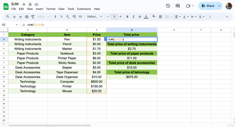
Close the cell
After specifying the range of numbers, close the function with a closing parenthesis ). The complete function will look like =SUM(A1:A10).
6. Press Enter
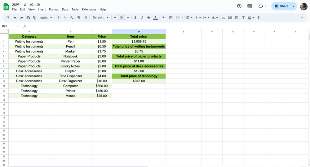
Press Enter
Once you've entered the function correctly, press Enter. The selected cell will display the total sum of the specified range of numbers.
💡If you want to learn how to use PERCENTILE function, check out our article.
What’s the difference between the SUM function and the SUMIF function?
Use the SUM function for the basic addition of numbers or values, and use the SUMIF function when you need to selectively sum numbers based on specific conditions or criteria within a given range of cells. The choice between these functions depends on the nature of your data and the desired outcome of the calculation.
Here are the key differences between SUM and SUMIF function:
Usage
- SUM: Used for straightforward addition of numbers or values.
- SUMIF: Used when you want to add numbers selectively based on specific conditions.
Conditions
- SUM: Does not involve conditions; it simply adds up specified numbers or values.
- SUMIF: Involves a condition (criterion) to determine which numbers to include in the sum.
Argument structure
- SUM: Accepts individual numbers, cell references, or ranges as arguments.
- SUMIF: Requires a range to evaluate, a criterion (condition), and optionally a sum_range (range to sum based on the condition
💡Do you know what the UNIQUE function is? Check our article!
Can I sum up data without using the function?
Yes, you can sum up data in Google Sheets without explicitly using the SUM() function in a formula bar. Here are the steps:
1. Select the cell where you want the sum to appear.
2. Click and drag to select the range of cells you want to sum.
3. Look at the bottom right corner of the selection. A small pop-up will appear with the sum of the selected cells. You can click on this pop-up to confirm the sum.
This method allows you to quickly see the sum of a range of cells without needing to type a formula explicitly in the formula bar. It is convenient for simple calculations and provides a visual way to verify the sum of your data.
However, keep in mind that for more complex operations or if you need to use the sum in a formula, using the SUM() function in the formula bar is usually the most flexible approach.
Frequently asked questions about the SUM function
In Google Sheets, you can use the AutoSum feature to quickly add up a column or row of numbers. The AutoSum feature in Google Sheets is similar to Excel's AutoSum functionality and allows you to automatically insert a SUM function for a selected range of cells. Here's how you can use AutoSum in Google Sheets:
- Select the Cell: Click on the cell where you want the total to be displayed.
- Initiate AutoSum: Press Alt + = on your keyboard or click on the Σ (sigma) icon in the toolbar.
- Confirm the Range: Make sure the selected range displayed by AutoSum covers the numbers you want to sum.
- Apply the Sum Formula: Press Enter to finalize and calculate the sum using the selected range.
To use the SUMIF function in Excel, follow these steps:
- Open Excel: Launch Microsoft Excel on your computer.
- Select the Cell for the Result: Click on the cell where you want the sum result to appear.
- Enter the Formula: Type =SUMIF( in the formula bar.
- Specify the Range: Enter the range of cells where you want to apply the condition. For example, if your data is in cells A1:A10, enter A1:A10.
- Enter the Criteria: Input the criteria based on which you want to sum the values. This can be a number, text, logical expression, or cell reference. For example, if you want to sum values greater than 50, you can enter ">50".
- Specify the Sum Range (if different from the range in step 4): If the range from which you want to sum values is different from the range used in the criteria, enter the sum range. For example, if the values to sum are in cells B1:B10, enter B1:B10.
- Close the Parentheses and Press Enter: Complete the formula by closing the parentheses and press Enter. Excel will calculate the sum based on the specified criteria.
The SUMIF function is a valuable tool available in Excel (and similar spreadsheet applications such as Google Sheets) that enables you to calculate the sum of values within a specified range based on specific conditions or criteria. This function is especially handy for conducting calculations on a subset of data that satisfies particular criteria within a larger dataset.
To sum only positive numbers in Excel, you can use the SUMIF function along with a criteria that filters out negative or zero values. Here's a step-by-step guide on how to do this:
1. Identify your data range: Determine the range of cells that contains the numbers you want to sum. Let's assume your numbers are in cells A1:A10.
2. Enter the SUMIF formula:
- Click on the cell where you want the result to appear.
- Enter the following formula:
=SUMIF(A1:A10, ">0")
- This formula will sum all positive numbers in the range A1:A10.
3. Understanding the formula:
- A1:A10: This is the range of cells containing the numbers you want to evaluate.
- ">0”: This is the criteria that specify you want to sum only numbers greater than zero (i.e., positive numbers).
4. Press Enter: After entering the formula, press Enter. Excel will calculate and display the sum of all positive numbers in the specified range.
Key points to take away
There are many Google Sheets formulas to make your work more effective, like the SUM function. The SUM function in Google Sheets computes the sum of a series of numbers or individual values. It is commonly used for basic arithmetic calculations within spreadsheet data, such as totaling a list of numbers or specific values.
This article covered the SUM function, its usage, and how it differs from the SUMIF function. You also learned how to automatically add numbers in Google Sheets, subtract in Google Sheets, and sum rows in Google Sheets. Now that you know how to use the formula, you can boost your power in Google Sheets!
Contributors
forms.app, your free form builder
- Unlimited views
- Unlimited questions
- Unlimited notifications
