How to use the COUNTIF function in Google Sheets

To effectively utilize the COUNTIFS formula in either Excel or Google Sheets, it's crucial to grasp its syntax. Breaking down its structure facilitates a thorough comprehension of its capabilities, facilitating efficient data analysis. Moreover, proficiency in the COUNTIF function within Google Sheets is of significant importance for a multitude of analytical endeavors.

In this article, you will learn about the COUNTIF function, its use, and how to apply it to Google Sheets. You will also find some answers to commonly asked questions. Let’s start with the definition!

What is the COUNTIF function?

The COUNTIF function in Google Sheets (and Excel) counts the number of cells within a range that meets a specified condition. 

You can use COUNTIF to count the number of cells that contain a certain value, are greater than a certain value, or match specific criteria.

When to use the COUNTIF function?

You learned what the COUNTIF function is. So, when to use this? You can use the COUNTIF function whenever you need to count the number of cells in a range that meets a specific condition. Some common use cases for the COUNTIF function include:

1. Counting the number of times a particular value appears in a range

2. Counting the number of cells that contain a certain text string

3. Counting the number of cells that meet a numerical condition (e.g., greater than, less than, equal to, etc.)

4. Counting the number of cells that meet a date or time condition

5. Counting the number of cells that match specific criteria using wildcards or logical operators

In summary, you can use the COUNTIF function whenever you need to quickly and easily count cells based on specific criteria within a range.

💡Do you know how to add a drop-down menu? Check our article and learn.

How to apply the COUNTIF function in Google Sheets

To apply the COUNTIF function in Google Sheets, follow these steps:

1. Open your Google Sheets document.

Open your Sheet

2. Click on the cell where you want the result to appear.

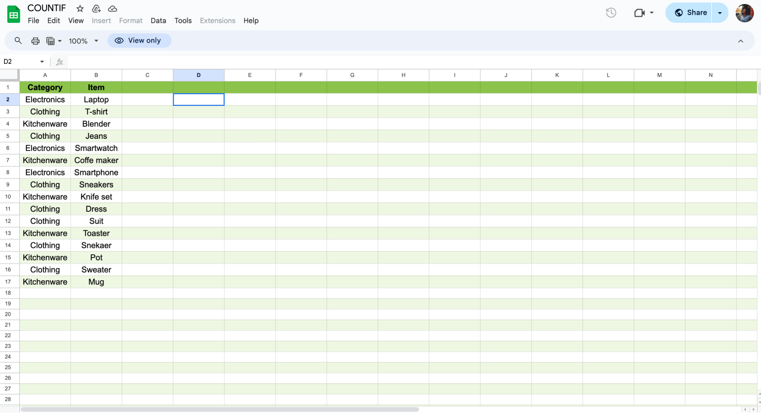
Click a blank cell

3. Type the formula =COUNTIF( into the cell.

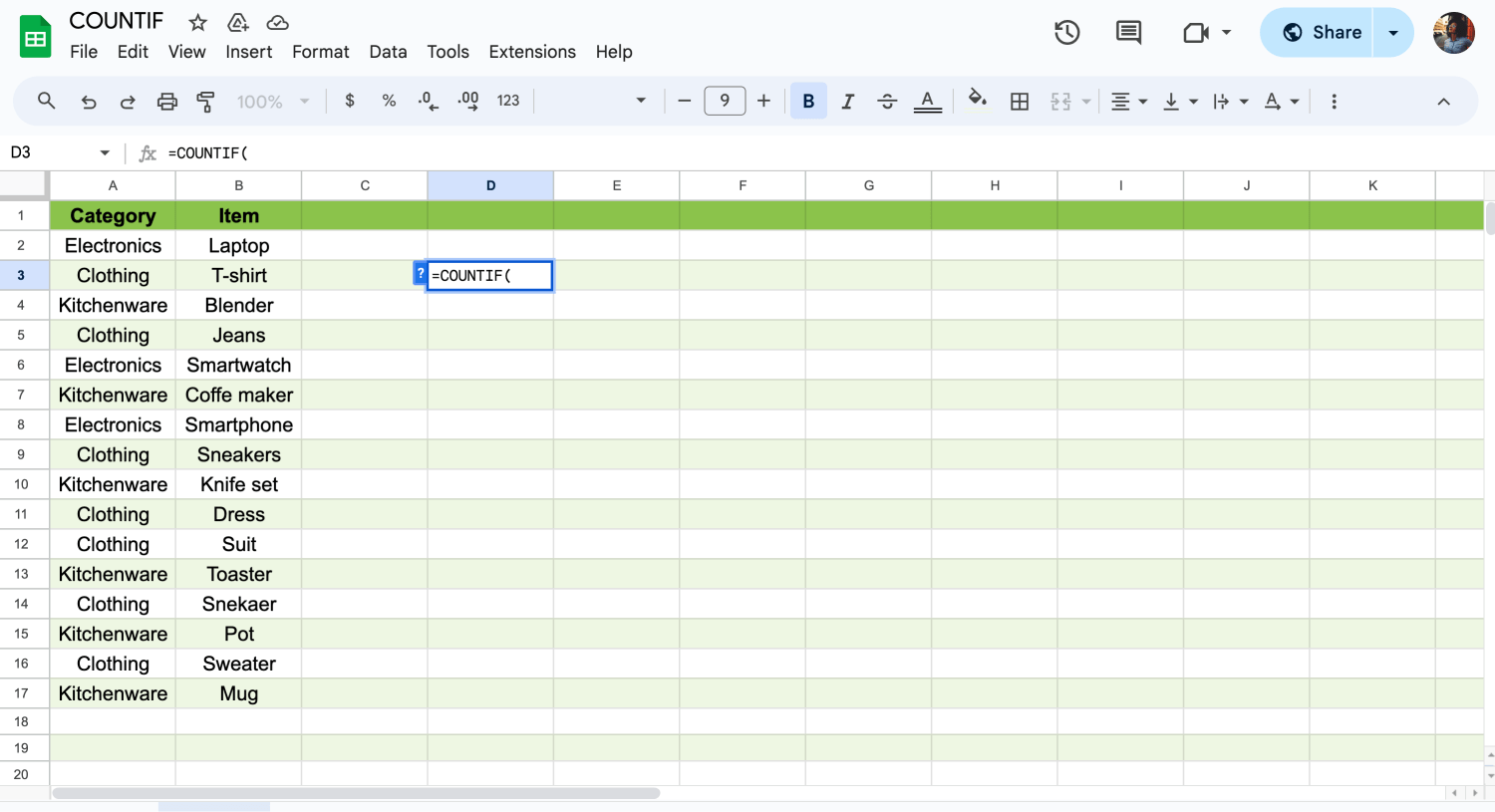
Start typing the formula

4. Specify the range of cells you want to evaluate. You can do this by clicking and dragging to select the range or manually typing the range, for example, A1:A17.

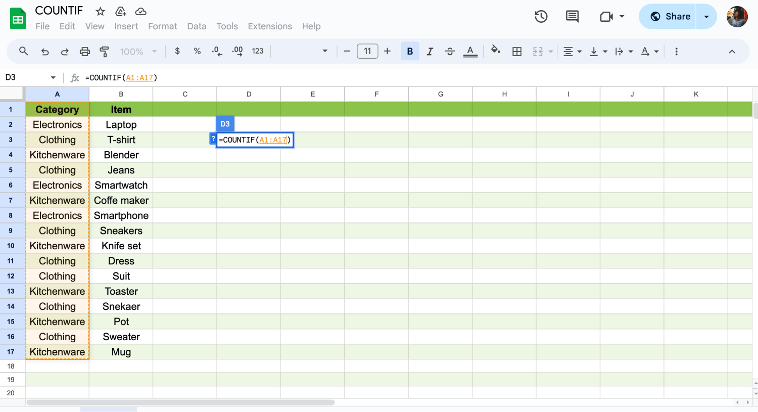
Choose the data

5. Type a comma (,).

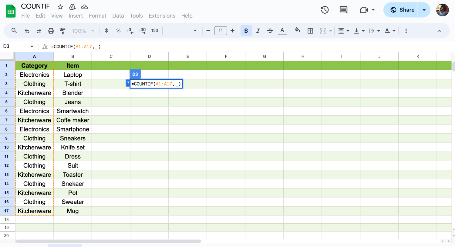
Don’t forget to type ','

6. Enter the criteria you want to count. This could be a specific value, text string, numerical condition, or date/time condition. Enclose text criteria in double quotation marks, for example, Electronics.

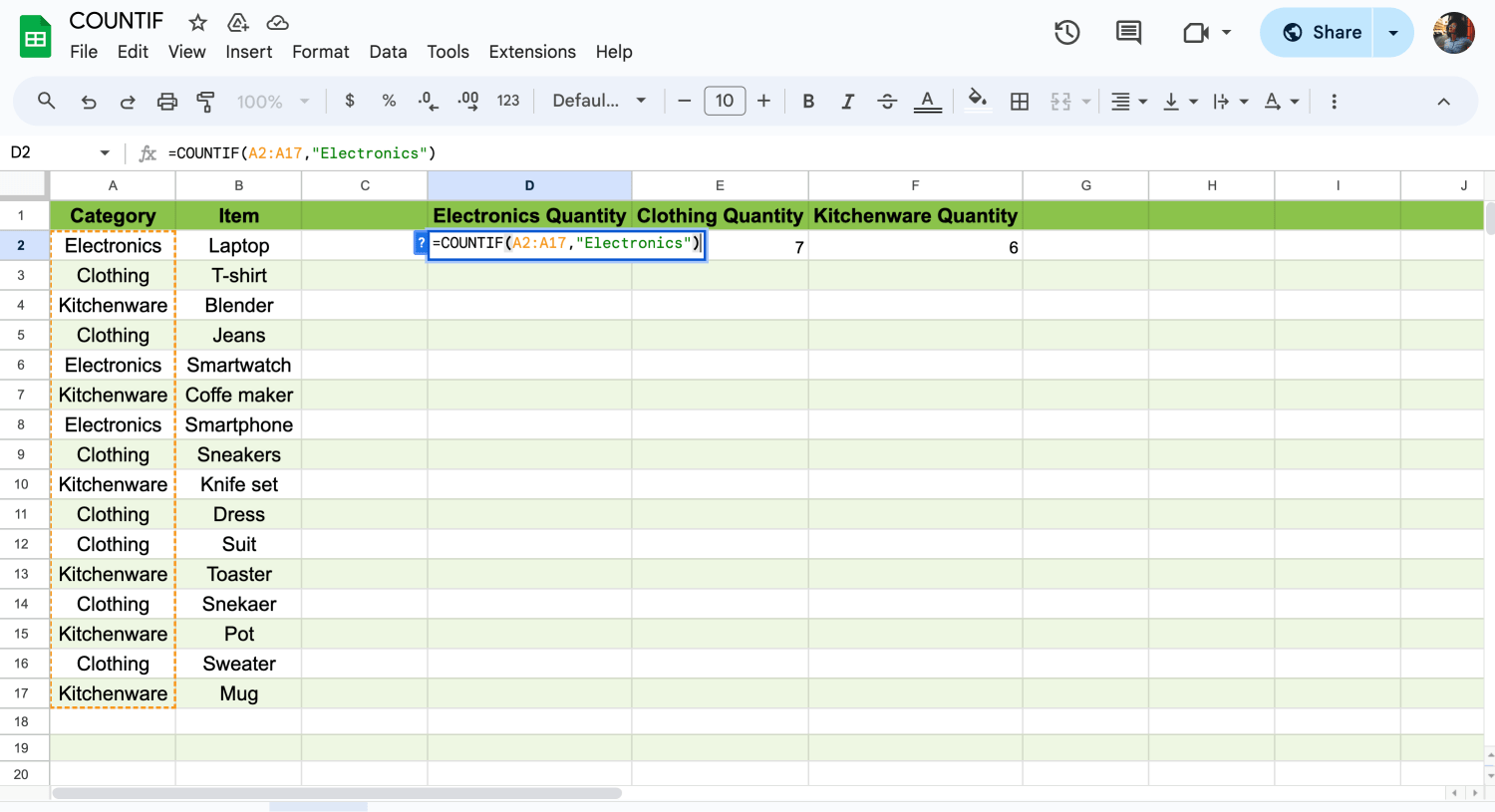
Complete the formula

7. Close the parentheses ) and press Enter.

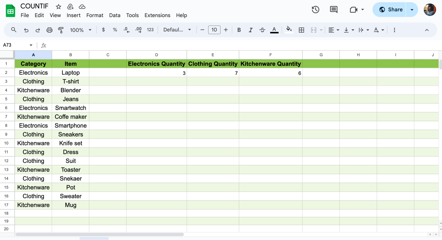
Apply the formula as much as you need

For example, if you want to count how many cells in the range A1:A17 contain the text ‘Electronics’, your formula would look like this:

=COUNTIF(A1:A17, ‘Electronics’)

Google Sheets will then calculate the count based on your specified criteria and display the result in the selected cell.

💡If you want to learn how to make an x-y graph in Google Sheets, check out our article.

Frequently asked questions about the COUNTIF function

You learned what the COUNTIF function is and how to use and apply it in Google Sheets at this point. If you want to learn more details about the COUNTIF function, you can read some commonly asked questions below.

Excel'de EĞERSAY işlevi nedir?

Bir ölçütü karşılayan hücrelerin sayısını saymak için istatistiksel işlevlerden biri olan EĞERSAY'ı kullanın; örneğin, bir müşteri listesinde belirli bir şehrin kaç kez göründüğünü saymak için.

En basit haliyle EĞERSAY şöyle der:

=EĞERSAY(Nereye bakmak istiyorsunuz?, Ne aramak istiyorsunuz?)

EĞERSAY’ı iki koşulla birlikte nasıl kullanırsınız?

=EĞERSAY(aralık1, kriter1, aralık2, kriter2)

- aralık1: İlk koşul için değerlendirmek istediğiniz hücre aralığı.

- kriter1: `aralık1` içinde karşılanması gereken koşul.

- aralık2: İkinci koşul için değerlendirmek istediğiniz hücre aralığı.

- kriter2: `aralık2` içinde karşılanması gereken koşul.

Örneğin, A ve B sütunlarında verileriniz olduğunu ve her iki koşulun da karşılandığı örneklerin sayısını saymak istediğinizi varsayalım:

1. Excel veya Google Sheets’te, sayım sonucunun görünmesini istediğiniz hücreyi seçin.

2. =EĞERSAY(A:A, "koşul1", B:B, "koşul2") formülünü girin.

3. "koşul1" ve "koşul2"yi sırasıyla A ve B sütunlarına uygulamak istediğiniz ölçütlerle değiştirin.

💡Google Sheets’te çizgi grafiklerin nasıl yapılacağı hakkında bilgi edinmek istiyorsanız yazımızı okuyabilirsiniz.

Değerler arasında EĞERSAY nasıl kullanılır?

Bir aralıktaki değerleri saymak üzere EĞERSAY fonksiyonunu kullanmak için gerektiğinde büyüktür (>), küçüktür (<), büyüktür veya eşittir (>=), küçüktür veya eşittir (<=) veya eşit değildir (<>) gibi karşılaştırma operatörlerini kullanarak kriterler belirleyebilirsiniz. İşte genel söz dizimi:

=EĞERSAY(aralık, ">değer1", aralık, "<değer2")

- aralık: Değerlendirmek istediğiniz hücre aralığı.

- ">değer1": Değer1`den büyük değerleri belirten koşul.

- "<değer2": değer2`den küçük değerleri belirten koşul.

Örneğin, A sütununda bir sayı listeniz varsa ve 10'dan büyük ve 20'den küçük sayıları saymak istiyorsanız:

1. Excel veya Google Sheets’te, sayım sonucunun görünmesini istediğiniz hücreyi seçin.

2. =EĞERSAY(A:A, ">10", A:A, "<20") formülünü girin.

Bu formül, A sütununda 10'dan büyük ve 20'den küçük olan değerlerin sayısını sayacaktır.

Benzer şekilde, gerektiğinde diğer karşılaştırma operatörlerini de kullanabilirsiniz. Ölçütlerdeki aralıkları ve değerleri özel gereksinimlerinize uyacak şekilde ayarlayın.

Eğersay ve eğer birlikte kullanılır mı?

Evet, EĞERSAY fonksiyonunu Excel veya Google Sheets’te EĞER fonksiyonu ile birlikte kullanabilirsiniz. Ancak kullanım tam olarak neyi başarmaya çalıştığınıza bağlı olarak değişebilir. Örneğin, belirli koşulları yalnızca başka bir koşul karşılandığında saymak isteyebilirsiniz. Bu durumda EĞERSAY fonksiyonunu EĞER fonksiyonunun içine yerleştirebilirsiniz.

EĞERSAY ve EĞER’i birleştirmek verilerinizi Excel veya Google Sheets’te analiz etmek ve işlemek için güçlü yollar sağlayabilir. Koşulları ve ölçütleri özel gereksinimlerinize göre ayarlayın.

Excel'de değer aralığı olan hücreleri nasıl sayabilirim?

Excel'de bir değer aralığındaki hücreleri saymak için birden çok ölçütle EĞERSAY işlevini kullanabilirsiniz. Bunu şu şekilde yapabilirsiniz:

=EĞERSAY(aralık, ">=başlangıç_değeri", aralık, "<=son_değer").

Aralık yerine saymak istediğiniz gerçek hücre aralığını, başlangıç değeri yerine değer aralığının alt sınırını ve `son değer` yerine değer aralığının üst sınırını yazın.

Örneğin, A sütununda bir sayı listeniz varsa ve 10 ile 20 arasındaki değerleri içeren hücreleri saymak istiyorsunuz:

=EĞERSAY(A:A, ">=10", A:A, "<=20")

Bu formül, A sütununda 10 ile 20 arasında değerler içeren hücrelerin sayısını verecektir.

Aralıkları ve değerleri özel verilerinize ve ölçütlerinize uyacak şekilde gerektiği gibi ayarlayın.

Final words

Understanding the syntax of the COUNTIFS formula is essential for proficient use in both Excel and Google Sheets. By dissecting its structure, one can gain a comprehensive understanding of its functionality, enabling effective data analysis. Additionally, mastering the Google Sheets COUNTIF is crucial for various analytical tasks.

In this article, you delved into the intricacies of the COUNTIF in Google Sheets and explored how to use COUNTIF in Google Sheets. Now that you know each step, you can start utilizing the formula and boost your productivity!