The date plays a huge in saving data. So, recording data with a date in Google Sheets is important. At this point, Google Sheets date formulas and other menu extensions come to your rescue. If you want to learn how to put a date in Google Sheets or change it, keep reading.
In this article, you will learn how to change the date format in Google Sheets with the following easy methods. If you are looking for adequate Google Sheets time functions with excellent explanations, you will get what you want because we have gathered a complete guideway to change the date format in Google Sheets and more!
What is the default date format in Google Sheets?
The default date format in Google Sheets is the format that Google Sheets determines according to your location. For example, if you are a user from the UK, the default date format will be DD/MM/YYYY. However, if you are a user from North America, the default format will be MM/DD/YYYY.
In other words, the location that you exist in defines the default date format. As you wish, it is possible to change the date format. If you want to change the format but do not know how to, no worries because in our article, you will learn the process step by step.
How can I change the date format in Google Sheets?
The main question of our article is, “How can I change the date format in Google Sheets?” and it is possible to do it in various ways. You can change the format on the menu extensions or by using some functions in Google Sheets. So, you have 5 options for custom formatting, and here are them:
Method 1: Date format in the format menu
If you do not want to use any date function in Google Sheets, you can simply use this method. This method is pretty easy to use because it requires no formula. If you need to change your date format without applying a function, here are the steps:
1. Select the data you want to change.
2. Choose Format from the upper left corner. Then click the 123 - Number button from the extension.
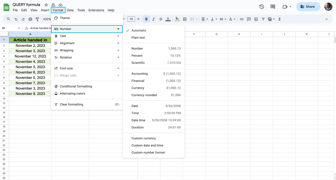
Opening the number section under format in Google Sheets
3. Choose any format you want from date time to duration.
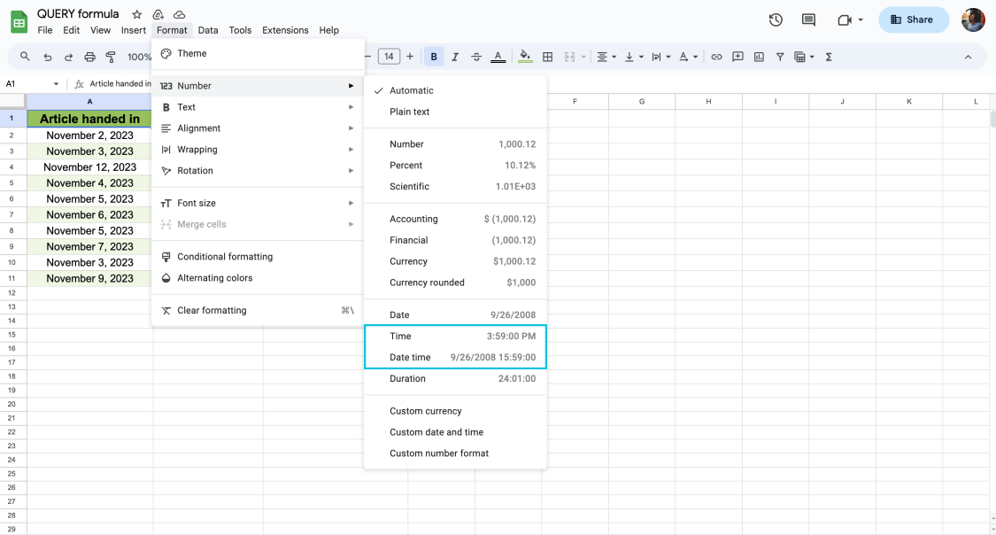
Number options for date, time, date time, and duration in Google Sheets
💡 You can also find the 123 Number button from the toolbar easily.
Method 2: DATEVALUE function
Using the DATEVALUE function method is a useful Google Sheets date function. The formula creates a date you want with the selected format. The DATEVALUE function is a handy Google Sheets date format formula for you to use in dates. Check the steps given below:
1. Select the cells you want to apply the formula.
2. Type =DATEVALUE(value) and press enter.
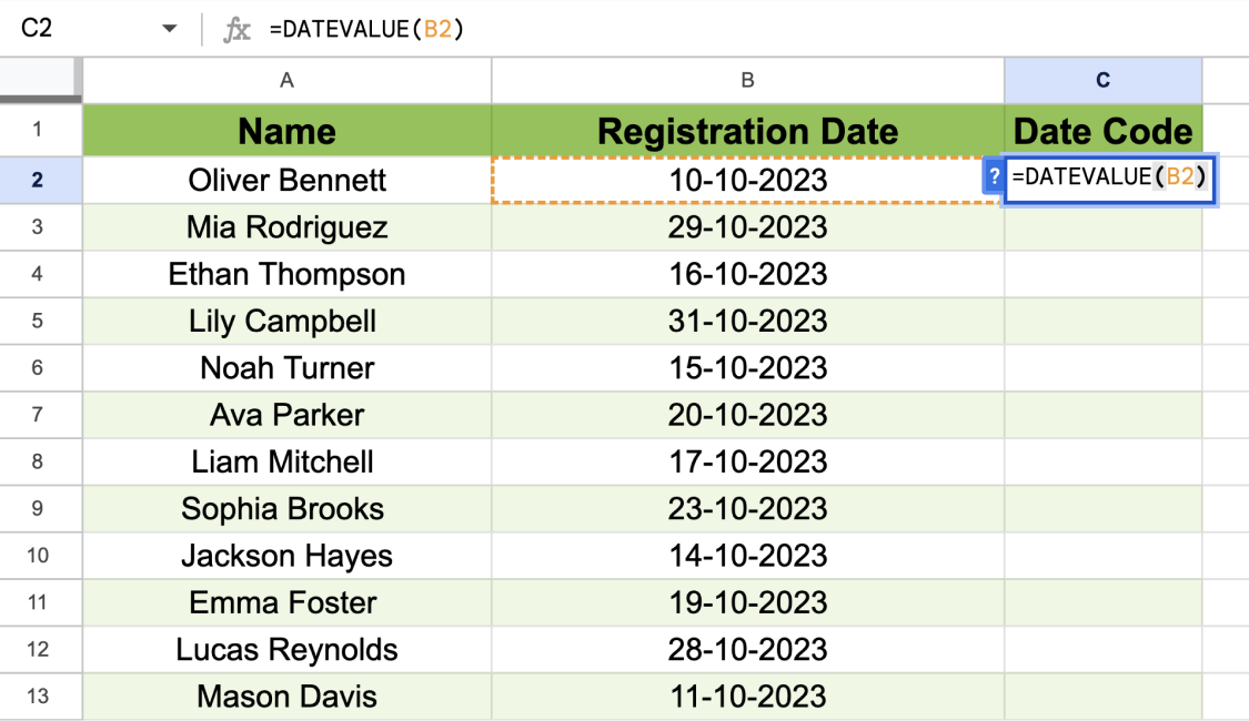
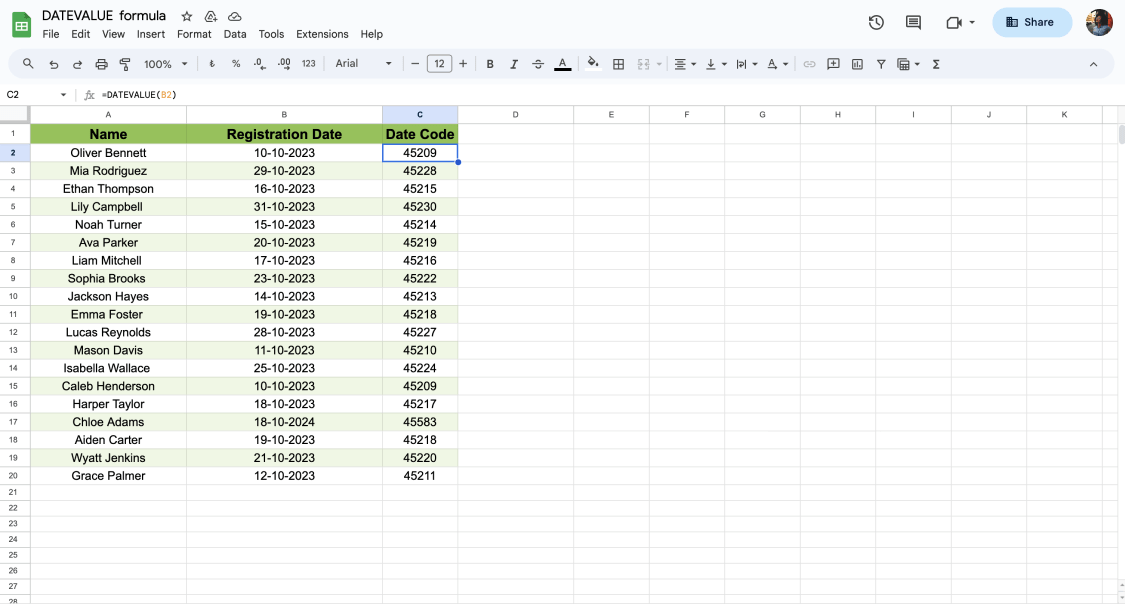
3. For example, if you type =DATEVALUE(B2), which consists of “10-10-2023”, you will get 45209, which represents the serial number of the cell B2.
💡 If the DATEVALUE function is not working properly, be sure that your locale and time zone are set correctly.
Method 3: TEXT function
The TEXT formula transforms numbers into texts, including currencies, dates, decimals, or other formats. It is mainly used in dates. If you need such a formula, follow the steps given below:
1. Click on any blank cell.
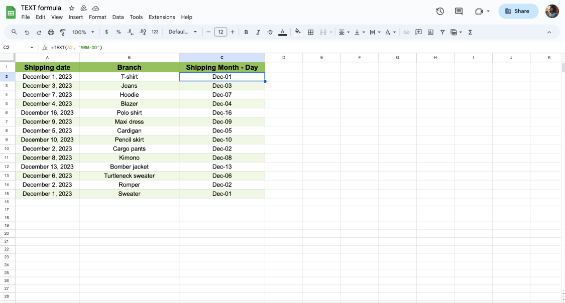
2. =TEXT(A2, "MMM-DD") for a cell that contains “December 1, 2023”; it will give you only the day, which is Dec-01.
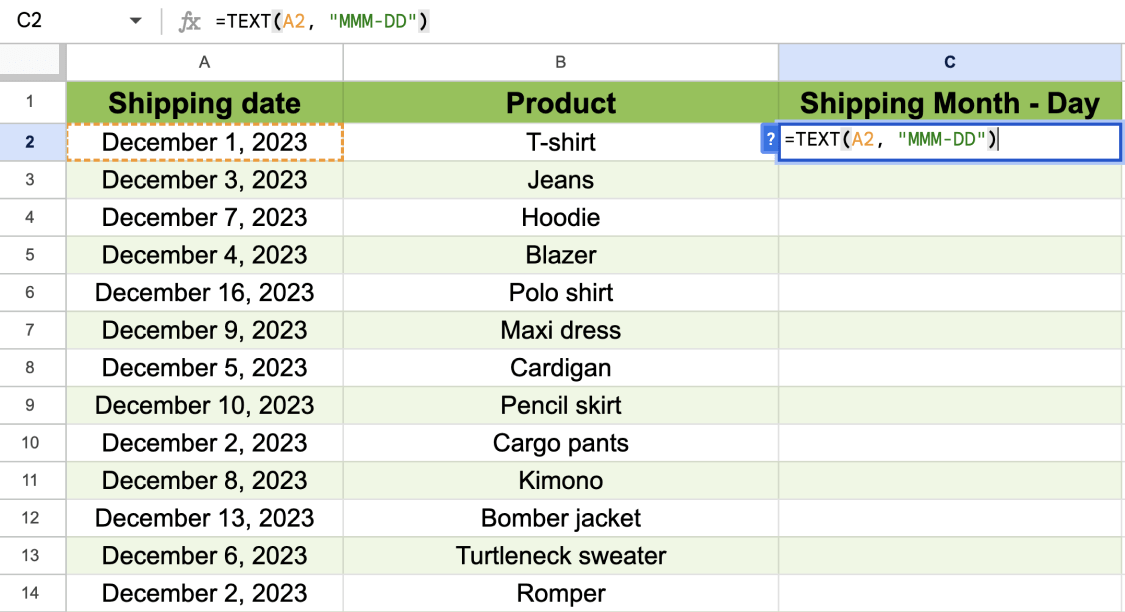
3. If you type =TEXT(A2, "dd mmm yy"), it will give you the month in text and the other details in numbers. Just drag the little ball on the bottom right corner to apply this formula to other cells.
💡The TEXT function is great for date and time formatting for a specific format. Here are other formatting abbreviations you can use.
‣ d: the day expressed as one or two digits (e.g. 5)
‣ dd: the day expressed as two digits (e.g. 15)
‣ ddd: short name of the day of the week (e.g. Mon)
‣ dddd: full name of the day of the week (e.g Monday)
‣ m: name of the month as one two digits (e.g. 9)
‣ mm: name of the month as two digits (e.g. 10)
‣ mmm: short name of the month (e.g. Dec)
‣ mmmm: full name of the month (e.g. December)
‣ yy: year as last two digits (e.g. 23)
‣ yyyy: year as four digits (e.g. 2023)
‣ h/hh: AM/PM hour clock (e.g. 1:05 PM)
‣ h/HH: 24-hour clock (e.g. 13:05)
Method 4: QUERY function
Formatting the date, time, and number columns in Google Sheets is made easier for users using the Query function. The QUERY function returns the long dates into the ideal date format you wish. If you are curious about the function, have a look at the steps:
1. Choose the data you want to custom. (e.g., from cell A2 to A11)
2. Decide on how you want to custom date and time.
3. Type =QUERY(value1:value2,” SELECT * FORMAT A ‘DD-MMM-YYYY'”) and arrange the formula in Google Sheets according to your needs. Press the enter key to see the result.
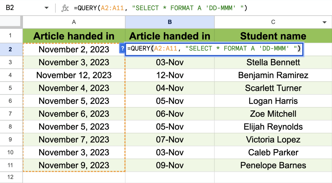
4. For example, if you type =QUERY(A2:A11, "SELECT * FORMAT A 'DD-MMM' "), you will see that the format will change from “November 2, 2023” to “02-Nov”.
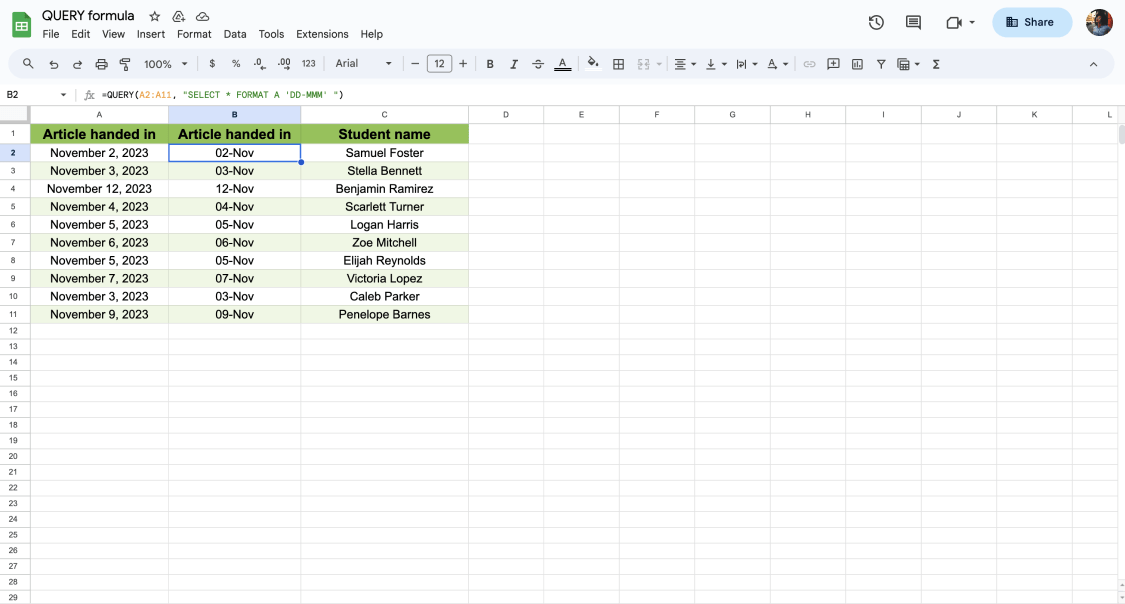
💡 You can change the day-month-year by checking the list we shared with you in the TEXT function section.
Method 5: Change the regional format
This method is another one that requires no formal to apply. As soon as you follow the basic instructions given below, you can change the format to another locale is really easy. To change the local from the toolbar, have a look at these steps:
1. Click File from the toolbar menu and click Settings.
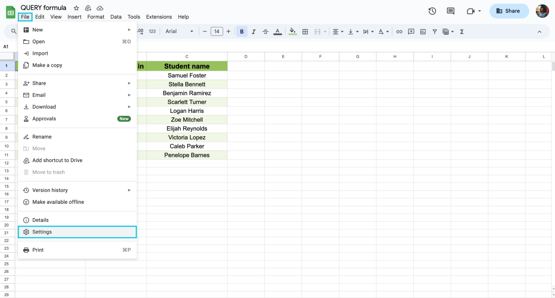
Opening the file settings
2. As you click, you will see both Locale and Time Zone.
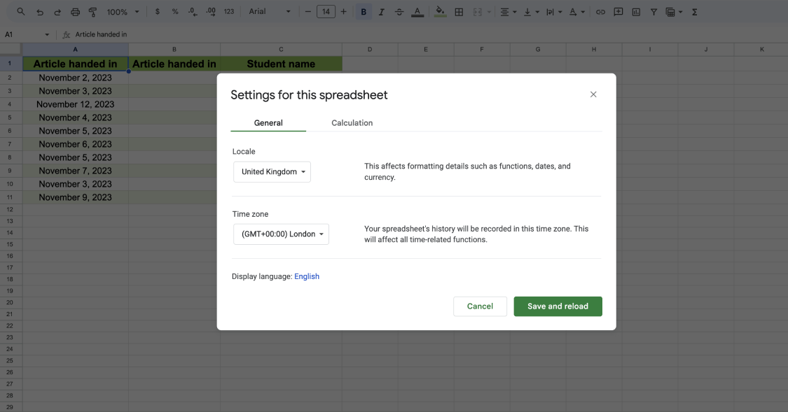
Finding the Locale and Time zone from settings
3. You can choose what you need, and after saving it, the date, year, month, and day will be according to your saved settings.
Frequently asked questions about the date format in Google Sheets
Even though we have explained how to change the Google Sheets format date as text or vice versa, you might still have questions about the issue. To help you find out more and find the answers to your questions, look at the frequently asked questions about the date format in Google Sheets given below:
As we have discussed so far, you have more than one option to change the date format in the spreadsheet from “MM DD YYYY” to “DD MM YYYY.” You can change the format and number of days by one of the methods below:
1. Changing date format from the Spreadsheet Settings.
2. Applying the DATEVALUE function.
3. Applying the TEXT function.
4. Applying the QUERY function.
5. Changing the locale to another.
Although the functions of Excel and Google Sheets are similar, you need to take different steps to change the date format in Excel. To change the date format in Excel to MMM YYY, you need to follow these steps:
1. Choose cells to format.
2. Press Command+1 or Control+1.
3. Click the Number Tab within the Format Cells box.
4. Click Date in the Category List.
5. Select a date format type from Type.
As we shared with you above, for Google Sheets, you can change the locale settings from the toolbar. For Excel, different steps need to be taken to change Europe and date to US date in Excel; you need to follow these steps:
1. Select the cells you want to change and click right.
2. Choose Format Cells, and from the window, you can easily change the locale from European to US.
3. Click OK and save your settings.
Yes, you can customize the date formats on the Google Sheets menu. If you check Method 1, you will see a detailed explanation for this question.
In Google Sheets, you can easily auto-fill the dates. All you need to do is click and hold the circle on the right corner of the cell and drag it. As you complete dragging, you will see that the cells will be automatically filled with the dates.
Your date might not be formatted in Google Sheets because of the locale settings. So, you might consider changing the locale time and zone. In Method 5, which we share above, you can learn how to change the date format to another locale.
In short
To wrap it all up, Google Sheets is an excellent tool for both individuals and businesses to save data. While saving the data, there might be moments when the date matters. At this point, it is essential to know the practical usage of Google Sheets formulas. You can learn more from our article about the best 20+ Google Sheets formulas to make your work easier. In our article, we aimed to guide you in changing the date format in Google Sheets with easy methods.
Şeyma is a content writer at forms.app. She loves art and traveling. She is passionate about reading and writing. Şeyma has expertise in surveys, survey questions, giveaways, statistics, and online forms.
