Thanks to Google Sheets, lots of businesses or companies save their data. The proper and effective usage of it saves lots of time. Google Sheets functions are excellent examples of this situation. If you want to make your work easier, keep reading because you will get what you want.
Formulas are excellent solutions for your business to increase the usability of Google Sheets spreadsheets. Formulas are like the magical language for Google Sheets, making it immediately more practical. In our article, you will learn 20+ of the best Google Sheets formulas to work like a pro!
What is a Google Sheets formula?
Google Sheets formulas are a mathematical language made by using an equal sign and starting a rule. Thanks to these formulas, you can arrange your data quickly. By adding specific numbers to your formulas, you can overcome complex tasks in a matter of seconds.
These formulas can be basic or complex; however, the main aim of both is to simplify, summarize, or categorize the data you select. So, as long as they are used correctly, Google Sheets formulas are a life-saver because they allow you to analyze an extensive range of data.
How to apply formulas for Google Sheets
Before starting right away, it is essential to know how to add formulas in Google Sheets. In order to apply formulas for Google Sheets, some steps need to be taken. As long as you follow the steps given below, you can start applying formulas for Google Sheets:
Before starting right away, it is essential to know how to add formulas in Google Sheets. In order to apply formulas for Google Sheets, some steps need to be taken. As long as you follow the steps given below, you can start applying formulas for Google Sheets:
1. Open your Google Sheets account and create a new spreadsheet.

Log in to your Google account
2. Click on any cell you want to add the formula
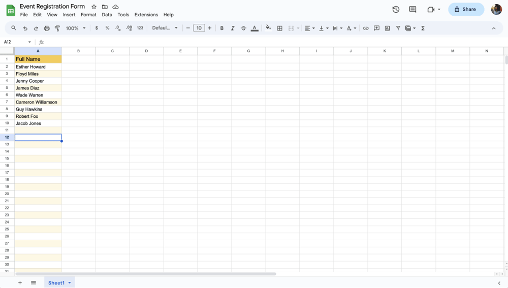
Clicking a cell on the spreadsheet
3. Choose the formula that you want or need to apply
4. Start typing “=” and continue typing your formula. It is the key part because without it, no matter how you pay attention to your formula, it will not work.
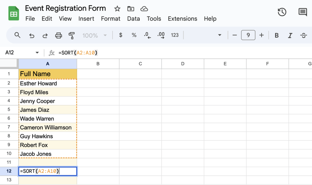
Appling a function on Google Sheets
5. Press enter to see the result
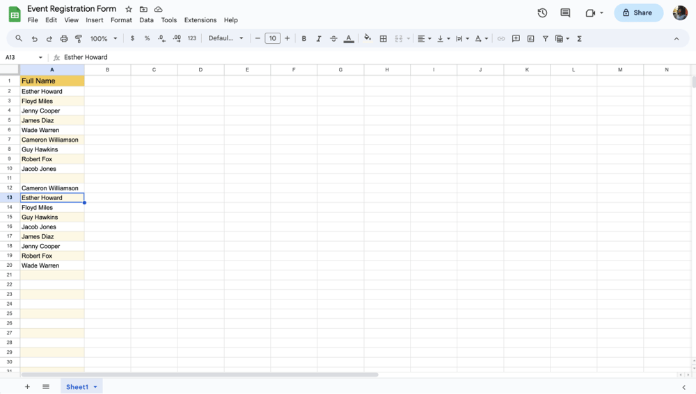
A spreadsheet showing the function results
20+ Google Sheets formulas to save time
Formulas save you an excellent amount of time and lighten your workload for sure. There are many formulas to use in Google Sheets; however, we have collected the most eye-opening ones to make your work easier. Here are the 20+ essential Google Sheets formulas cheat sheet for you:
1. SUM: adds the values
The SUM formula is one of the most used and common ones among the others. To find the sum, you can use the SUM formula to add various numerical values in the selected cells. All you have to do is:
1. Click on any blank cell.
2. Decide and select multiple cells you want to sum. Type: “=SUM(value1:value2)”
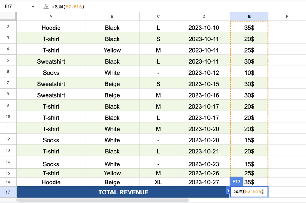
3. For example, type =SUM(E2:E16), press enter, and it will immediately give you the result.
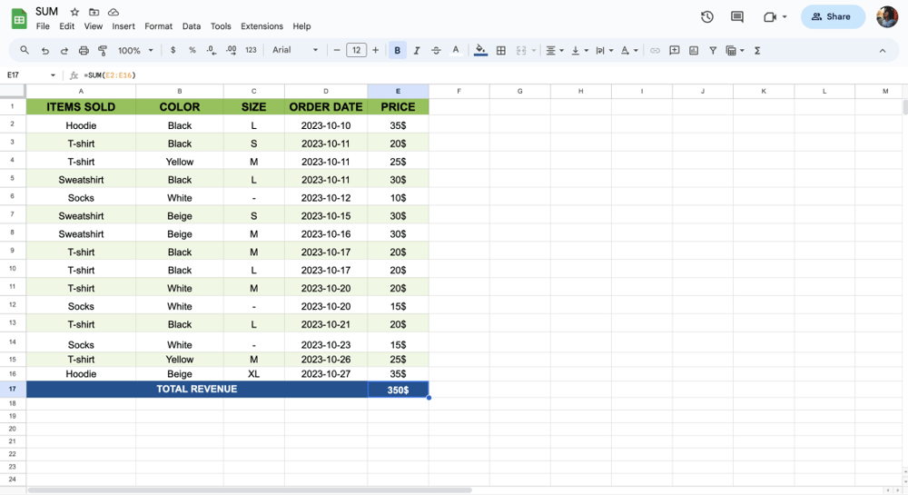
💡 If you have too much data that is hard to manage, you can easily sum up them via the SUM function.
2. SUMIF: sums of cells that meet definite conditions
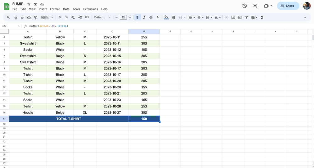
The SUMIF formula lets you determine the total number of cells that meet specific conditions. The difference from the SUM formula is that this formula also offers a chance to set specific criteria. Here are the steps to take:
1. Click on any blank cell.
2. Decide on the cells you want to carry out the formula and type: =SUMIF (range, criterion, [sum_range])
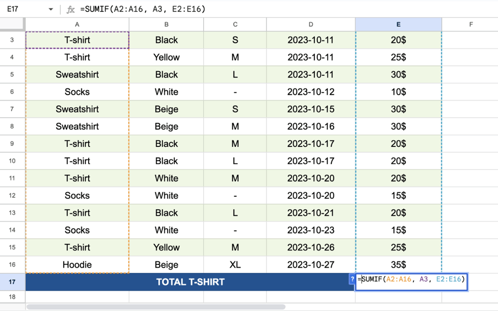
3. For example, type =SUMIF(F2:F13, 72, G2:G13), press enter, and it will immediately give you the result.
3. SORT: puts data lists back in alphabetical or numeric order
By using the SORT formula, you can easily sort cells from lowest to highest values. It also allows you to rearrange lists of your data according to alphabetical order. If you are wondering how here are the steps:
1. Click on any blank cell and type =SORT(value1: value2)
2. For example, if you type =SORT(A2:E16) and press enter, you will see the new column.
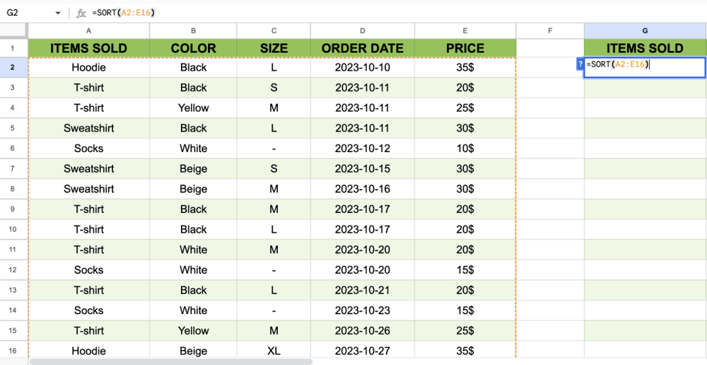
3. In the new column, the names will be arranged alphabetically.
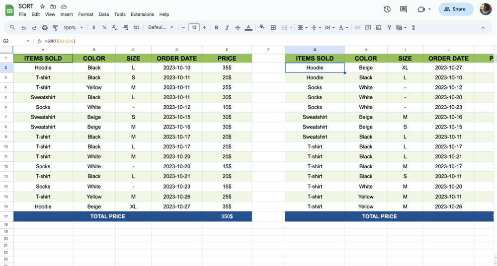
💡 If you need an alphabetical order to manage your data easier, you can use the SORT function.
4. TEXT: transforms numbers into texts
The TEXT formula transforms numbers into texts, including currencies, dates, decimals, or other kind of formats. It is especially used in dates. If you are in need of such a formula, follow the steps given below:
1. Click on any blank cell.
2. To illustrate, when you type =TEXT(value,"dddd") for a cell that contains “2023-10-26”, it will give you only the day, which is Thursday.
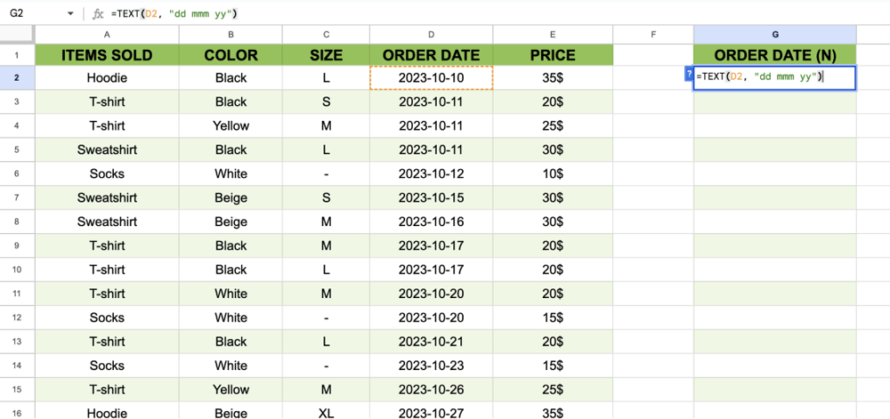
3. However, if you type =TEXT(D2, "dd mmm yy"), it will give you the month in text and the other details in number. Just drag the little ball on the bottom right corner to apply this formula to other cells.
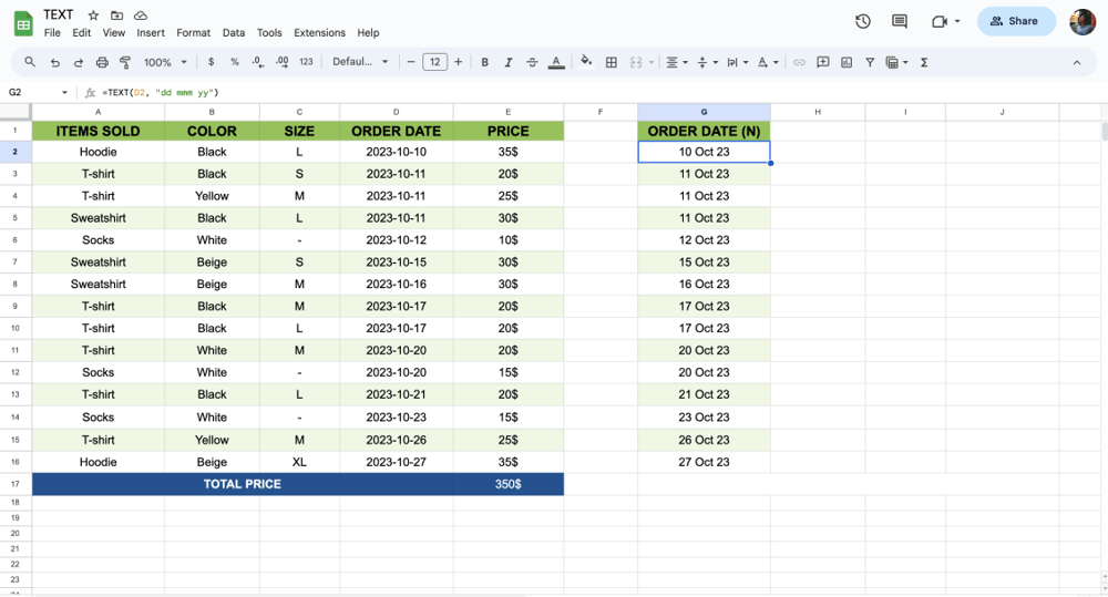
💡The TEXT function is great for formatting any numbers in a specific format. Here are other formatting abbreviations you can use.
d: the day expressed as one or two digits (e.g. 5)
dd: the day expressed as two digits (e.g. 15)
ddd: short name of the day of the week (e.g. Mon)
dddd: full name of the day of the week (e.g Monday)
m: name of the month as one two digits (e.g. 9)
mm: name of the month as two digits (e.g. 10)
mmm: short name of the month (e.g. Dec)
mmmm: full name of the month (e.g. December)
yy: year as last two digits (e.g. 23)
yyyy: year as four digits (e.g. 2025)
h/hh: AM/PM hour clock (e.g. 1:05 PM)
h/HH: 24-hour clock (e.g. 13:05)
Also, by adding 0 to the TEXT formula, you can change the numbers’ formats. To illustrate, if you type =TEXT(11.46, “0000.0000”), you will get 011.460.
5. COUNTA: determines the number of values put into a set
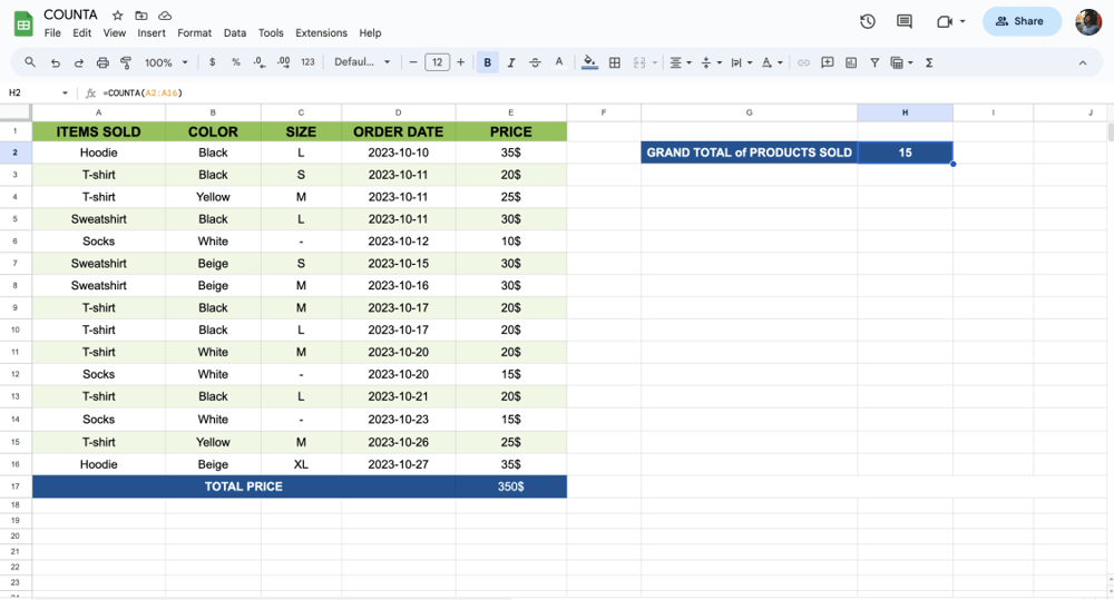
The COUNTA formula determines the number of values put into a set. If you need to know how many data are in each column, this formula will be helpful for you. Here are the steps you should follow:
1. Click on any blank cell. Type: =COUNTA(value1: value2)
2. To give an example, if you are wondering how much data you have entered in Column A, all you need to do is type =COUNTA(A2:A16)
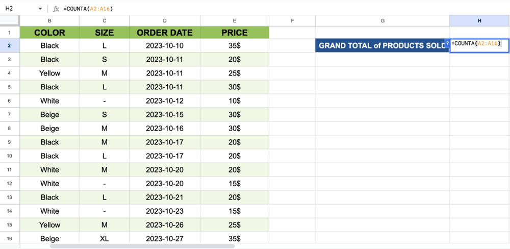
3. After entering the formula, you can see the total number entered in cells.
6. COUNTIF: specifies the range that you want to search
If specific criteria are met, the COUNTIF formula lets you count the number of cells. The COUNTIF formula allows you to select a non-numerical condition, much like the SUMIF function. Check the steps:
1. Decide on the cells you want to carry out the formula and click on any blank cell.
2. Type =COUNTIF(A:A,"Text")
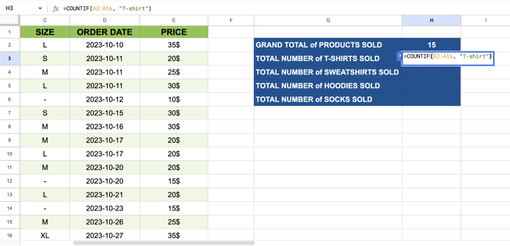
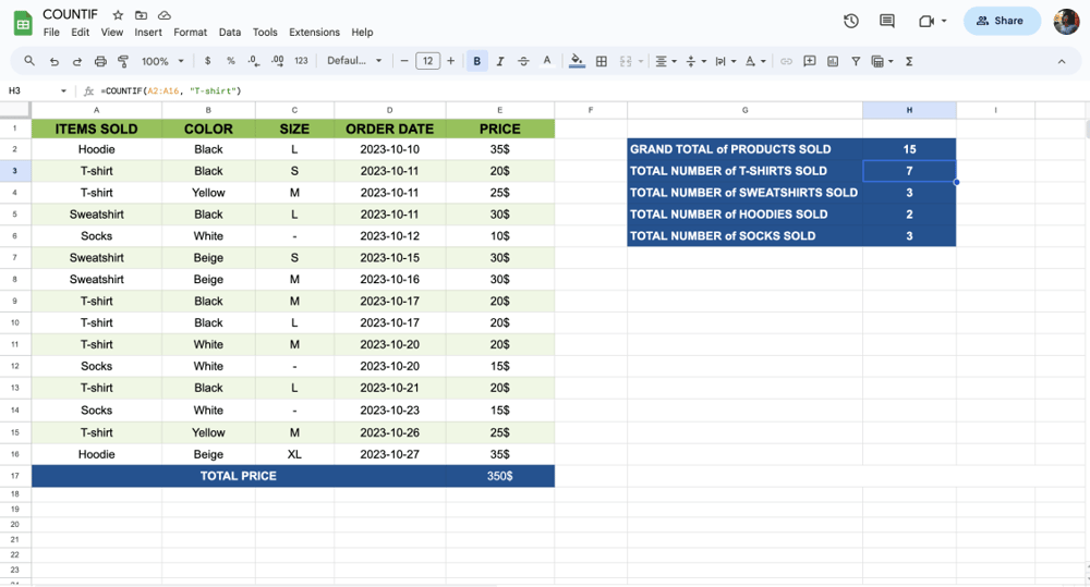
3. For instance, let’s assume you want to check how many T-shirt orders you have; all you need to do is type =COUNTIF(A2:A16, "T-shirt") and press enter. After that, you will see how many “T-shirts” they ordered.
7. SPARKLINE: enables you to construct an overview chart neatly fitting into a single-cell
This formula is an excellent tool for seeing a basic chart about the data you want. Column charts and single-cell bar charts are among the possible varieties for you to use. If you need these types of charts in your Google Sheets, you need to follow these basic steps:
1. Click on any blank cell and decide which cells you want to create a column.
2. You need to type =SPARKLINE(value1: value2)
3. To illustrate, if you want to see a chart in a single cell, you type =SPARKLINE(A2:G2)
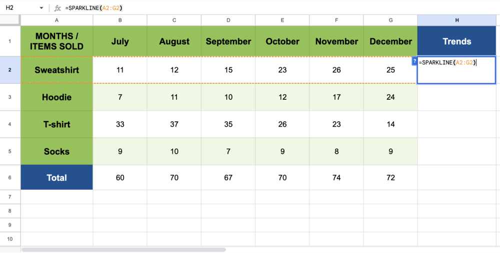
4. When you press the enter key, you will see a small chart in the cell.
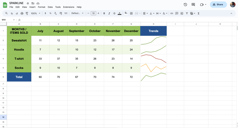
💡You can add extra details by editing the following formula additions and using them in your formula:
{"color","#599613"}
{"linewidth",2}
{“charttype”,”bar”}
{“charttype”,”column”}
{“charttype”,”winloss”}
E.g. =SPARKLINE(A2:G2,{"color","#599613";"linewidth",2})
8. MINUS: substracts the values
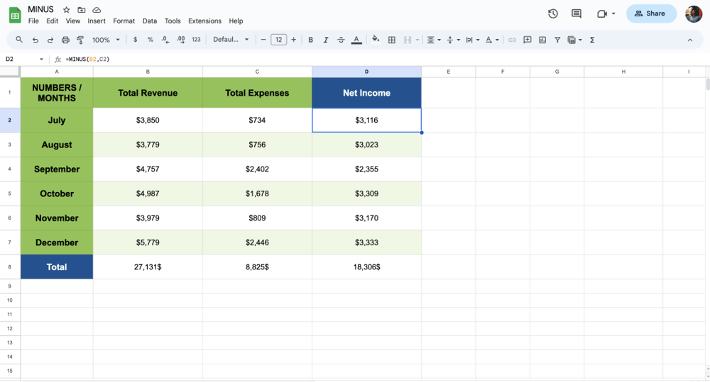
The MINUS formula is one of the most essential Google Sheets formulas to make your work much more manageable. Thanks to its non-complex formula syntax, you can immediately get your result. To perform calculations quickly, do the following:
1. Decide on the cells you want to make calculations and click on any blank cell.
2. Type =MINUS(value1, value2)
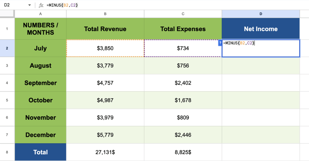
3. For example, you can type =MINUS(B2,C2), and it will automatically give you the result.
9. MIN: finds the lowest value
You can use the MIN function to determine the lowest value in a given range of cells. By using its simple and non-complex syntax, you can use the MIN formula to find the minimum value of the given cells. Follow these steps:
1. Click on any blank cell.
2. To learn, type =MIN(value1:value2)
3. To give an instance, you need to type =MIN(B2:B7)
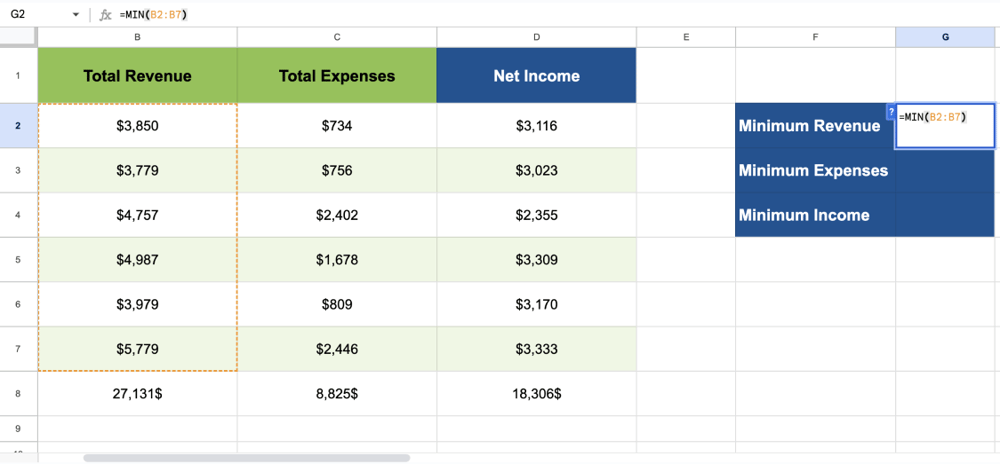
4. Press enter, and it will show you the lowest value.

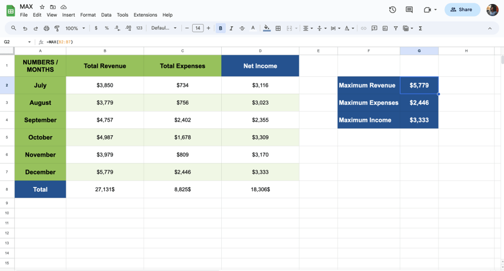
10. MAX: finds the highest value
Just like the MIN formula, the MAX formula has the same function, but the difference is that this one finds the highest value in a given range of cells. As long you apply the basic formula, you can easily apply the formula, and here it is:
1. Click on any blank cell, and to learn, type =MAX(value1:value2)
2. For example, type =MAX(B2:B7)

3. Press enter, and it will show you the highest value.
11. SPLIT: lets you divide contents from one cell into many
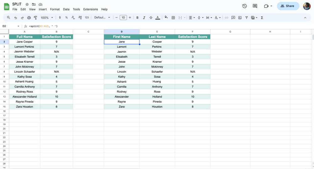
The SPLIT formula divides the next around a given string or character and then puts each aspect into a different row of cells. If you want to split a range of cells in your sheet, you need to apply this formula, and here are the steps:
1. Click on any blank cell. Let’s assume that you want to separate name and surname. You need to type =SPLIT (Value, " ")
2. For example, you want William and Swift in separate cells instead of a single cell. You need to type =SPLIT (A2:A15, " ")
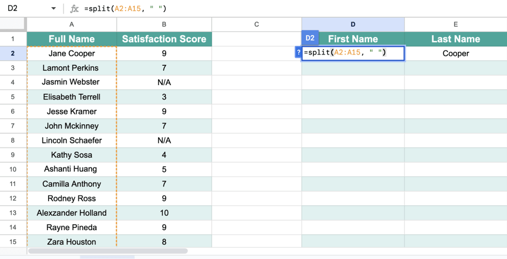
3. After you press enter, you will realize that the formula will separate the name into different rows and columns.
12. JOIN: combines different rows and cells into a singular cell
In contrast to the SPLIT formula, the JOIN formula combines different browns and cells into a singular cell. If you want to group a range of cells in your sheet, you need to apply this formula, and here are the steps:
1. Click on any blank cell. Let’s assume that you want to separate name and surname. You need to type “=JOIN (" ", values)
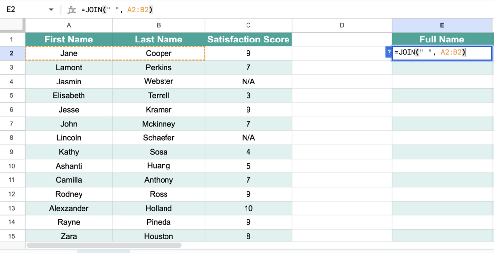
2. For example, you want first and last names in the same column instead of separate columns. You need to type =JOIN(" ", A2:B2). Once you press enter, you will see that the formula will immediately unite the cells.
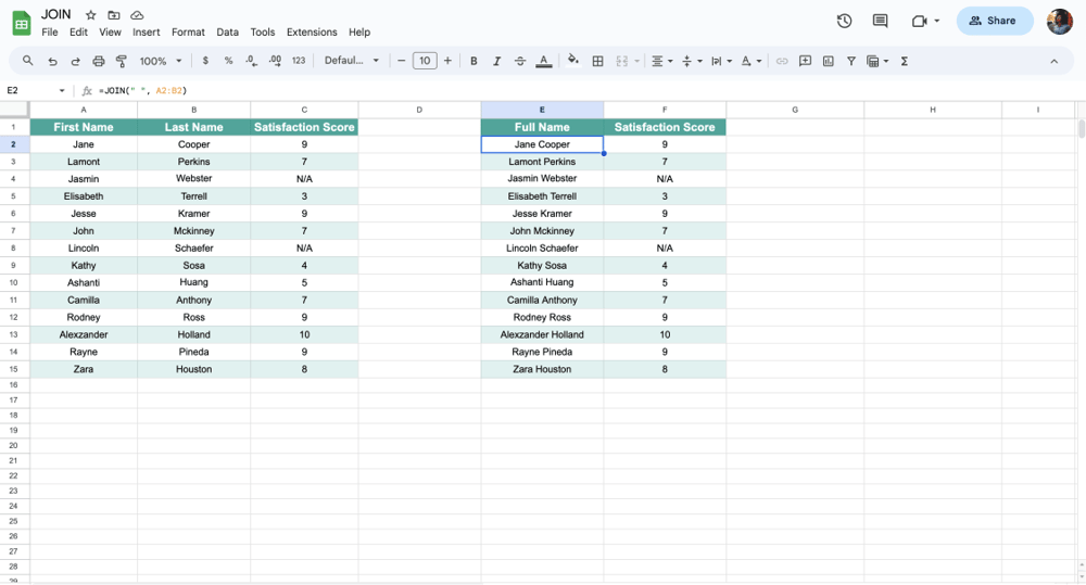
💡 When you type =JOIN (" ", values), the results will have a space between the values. However, if you type =JOIN ("", values), there will be no space between the values.
13. COUNT: gets the number of data in selected cells
To find out how many cells in a range contain a value, you need to use the COUNT formula. In other words, the number of entries in several fields that are inside a range may be obtained by using the COUNT function. Have a look at these steps:
1. Click on any blank cell and decide on the cells you want to count.
2. Type =COUNT(value1 : value2)
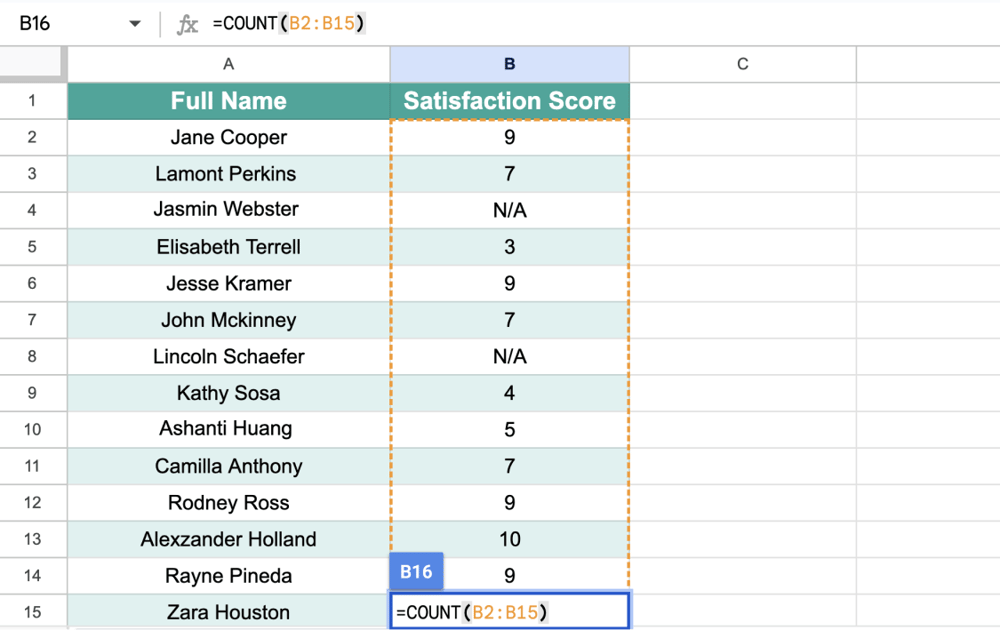
3. For instance, there might be blank cells between C2 and C14. To check, type =COUNT(B2:B15) and press enter.
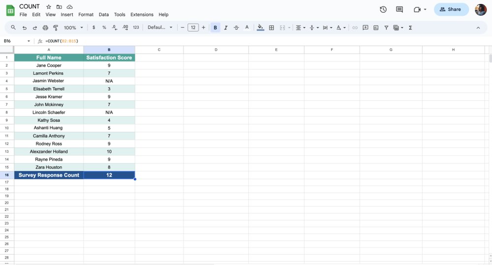
💡The difference between COUNT and COUNTA is: the COUNT formula only counts the cells that contain numbers, while the COUNTA formula counts each non-blank cell in the table.
14. SUBSTITUTE: changes a specific word
If you need to make a change to a definite word that you have in a specific range in Google Sheets, this formula will help you save time. If you need something like this, you can use this formula instead of searching and replacing it.
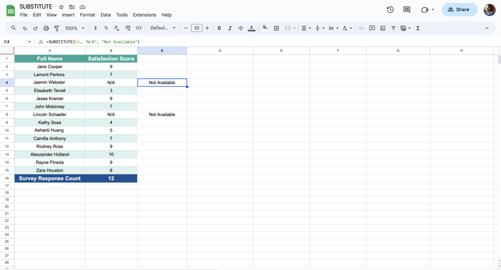
1. Click on any blank cell and Type =SUBSTITUTE(value, "old word", "new word")
2. To illustrate, if you want to change your word in A4, you need to change the formula as =SUBSTITUTE(B4, "N/A", "Not Available")
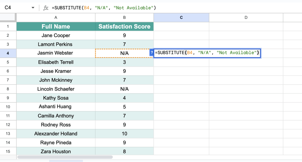
3. After you press enter, the word will change immediately.
15. NOW: finds the current time
If you want to learn and save the exact time, you need to use the NOW formula. It is really practical to use. Suppose that the data you save in Google Sheets matters regarding date and time. Then, you might need this formula. Read to learn how to use the formula:
1. Click on the blank cell you want to save the time and Type =NOW()
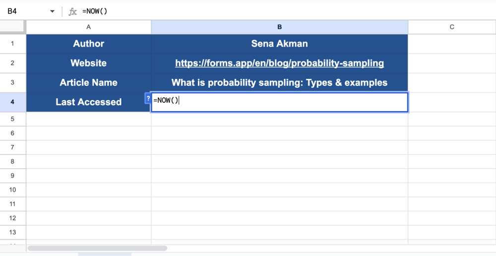
2. Press enter, and that’s all! You will see the exact date and time as soon as you apply the formula.
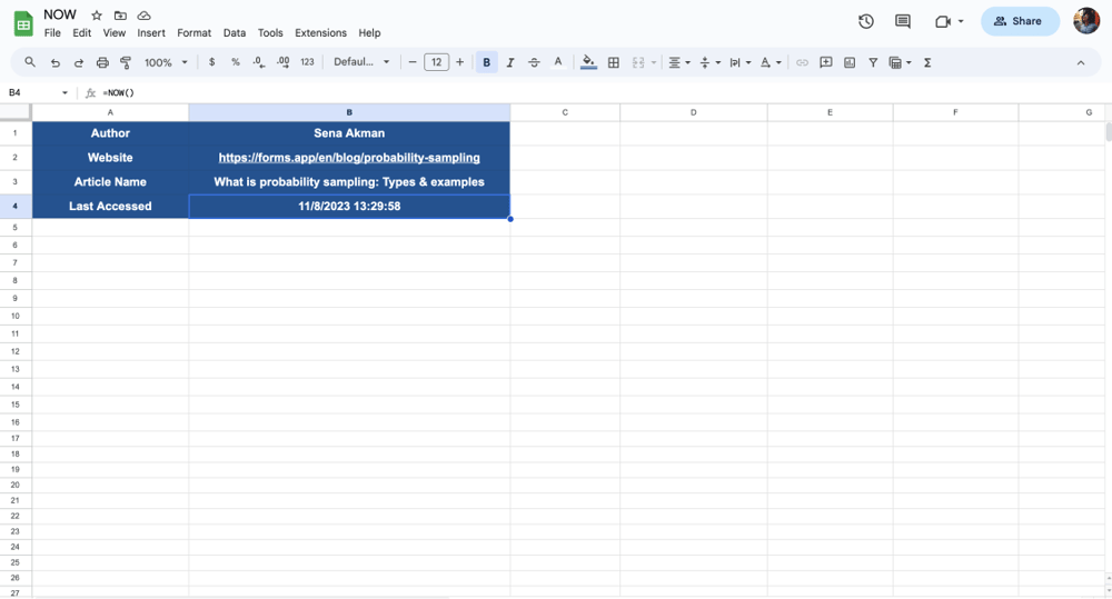
💡 If you need to take note of the time each time you enter data in Google Sheets, the NOW function will help you a lot.
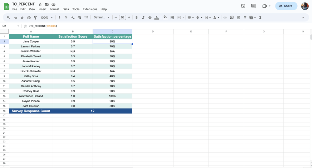
16. TO_PERCENT: turns values into percentages
The TO_PERCENT formula is when you want to learn the percentage of a value you want. The formula basically calculates the percentage of the value without your bothering. If you need this formula, apply these steps:
1. Find the rows and columns of the value you want to find the percentage and click on any blank cell.
2. Type =TO_PERCENT(value)
3. For instance, you need to type =TO_PERCENT(B2:B15)
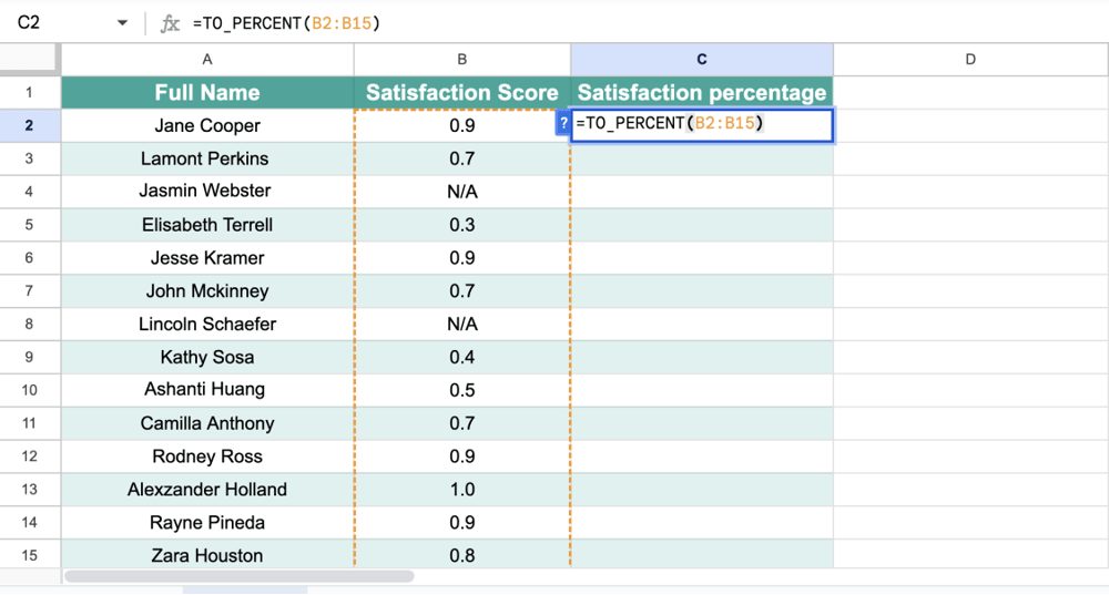
4. Press the enter key, and you will see the percentage.
17. MULTIPLY: multiplies the values
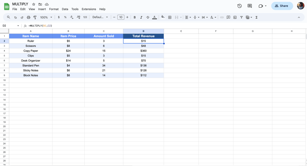
If you need or want to multiply two numbers, you can use the MULTIPLY formula. After you find out the correct cell references, you can quickly apply this formula. Here are the steps to take for this formula:
1. Click on any blank cell and decide on the correct cell reference.
2. Type =MULTIPLY(value1,value2)
3. =MULTIPLY(B2,C2) would be an example of this formula.
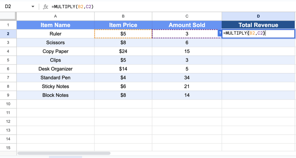
4. After pressing the enter, you will see the result.
18. DIVIDE: divides the values
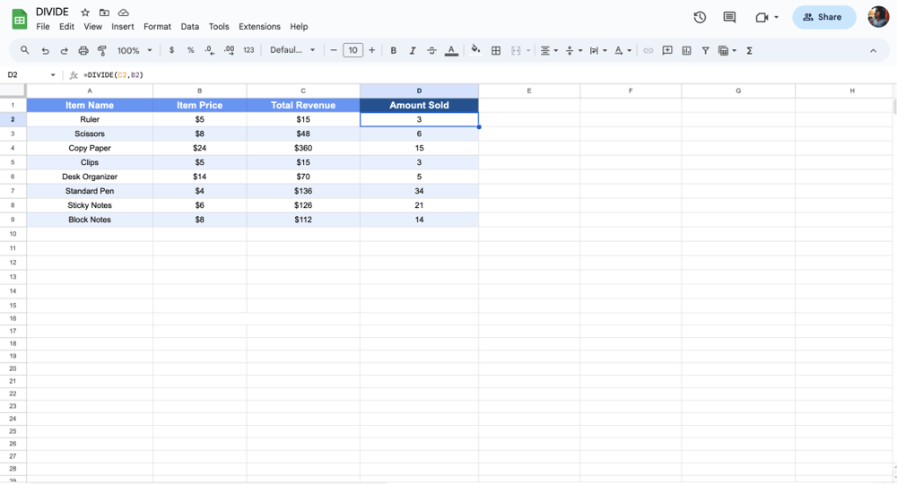
Just like the MULTIPLY formula, the divide has a similar function, except for its power of dividing. The formula lets you divide one value into another. If you need to apply this formula, you need to follow these steps:
1. Click on any blank cell and decide on the correct cell reference.
2. Type =DIVIDE(value1,value2)
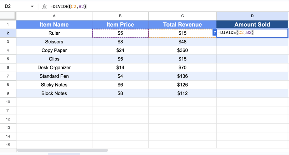
3. For instance, you will see the result as you type =DIVIDE(C2,B2)
19. DETECTLANGUAGE: detects the language
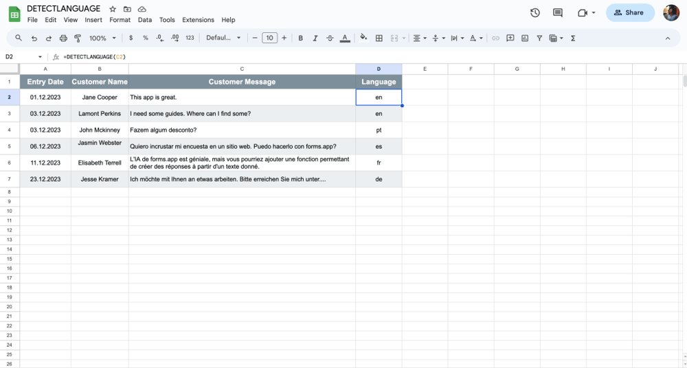
When you have a word you are alien to in your Google Sheets, and you do not know what language it is, you can use this formula. the DETECTLANGUAGE formula is really simple to apply and useful in such cases. Have a look at the steps:
1. Decide which word you want to learn via the formula and click on any blank cell.
2. Simply type =DETECTLANGUAGE(value)
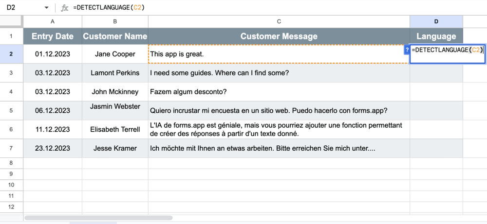
3. For example, if there is an unknown alphabet and you need to learn the language, you can type =DETECTLANGUAGE(C2) and press enter.
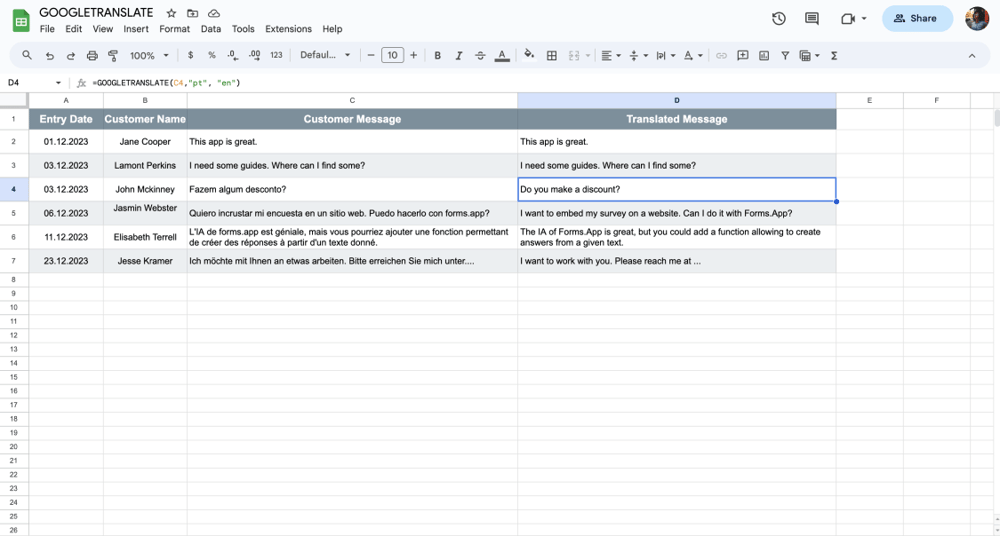
20. GOOGLETRANSLATE: translates texts
Did you know you can make translations directly on Google Sheets? It’s possible, and what’s more, it’s so easy. Simply follow the steps below:
1. Have your table ready and click on a blank cell.
2. Simply type =GOOGLETRANSLATE(Text, [From_language, To_language]).
3. For example, if there is an unknown alphabet and you need to learn the language, you can type =GOOGLETRANSLATE(C4,"pt", "en") and press enter.
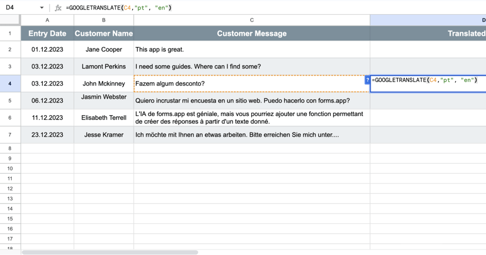
4. After pressing the enter key, you will learn the language.
Why are Google Sheets formulas essential?
As we have discussed so far, the formulas of Google Sheets are a real lifesaver. Google Sheets formulas arrange your imported data quickly as soon as possible. As long as they are used correctly, you can take advantage of the formula’s pros which will make your job easier. For the reasons listed below, Google Sheets formulas are really essential:
- Check the data you have entered
- Simplifies your spreadsheet
- Change the data you have entered
- Calculate the values easily
- Speeds up the process
- Makes the functions less complicated
Frequently asked questions about Google Sheets formulas
In this section of our article, we will discuss the frequently asked questions (FAQs) about Google Sheets formulas in order to help you. If you have any questions about the issue, you can check the question list given below and find the answers to it. Have a look at these FAQs about Google Sheets formulas:
Although Google Sheets and Microsoft Excel have different features, you can use most of the formulas on both of them. This means that you do not need to apply different formulas to your spreadsheet. The formulas we shared with you above can be applied to both.
All the formulas we shared above can be used in your Google Sheets. Each of the formals has different functions. According to your needs, you can choose one and apply them. The most important thing is not to forget “=” on each formula.
Yes, Google Sheets cells can have more than one formula. This situation is also known as the “nested formula.” To give an example, you can use the SUM function and the AVERAGE formula at the same time, which will give you the sum and average of the values you enter at the same time.
Yes, there is a kind of limit to the Google Sheets formula. Google Sheets has complexity limits. If the formula is too complicated, Google Sheets might not give you the correct answer, or it might take too much time. So, you might pay attention to simplifying your formula as soon as possible.
There are some operators used in Google Sheets commonly. In the following list, you can find some operators that Google Sheets knows:
- + : add
- - : subtract
- * : multiply
- / : divide
^ : exponentiate
Key points to take away
In short, Google Sheets makes our workload much lighter. Especially when we combine Google Sheets and formulas, they make our jobs much easier by creating perfection. In our article, we have shared the best 20+ Google Sheets formulas that will work you like a pro and save you time with explanations, frequently asked questions, and more.
If you want to get down to business without losing time, you can start applying these formulas on your Google Sheets right away!
Contributors
forms.app, your free form builder
- Unlimited views
- Unlimited questions
- Unlimited notifications
