How to use the SUMIF function in Google Sheets (Easy guide)

The SUMIF function in Google Sheets is an essential tool for anyone managing large datasets. You can sum up a range of cells based on specific criteria. This makes data analysis faster and more efficient. By using the SUMIF function, you can simplify many of your daily tasks.

In this guide, you will learn how to use the SUMIF function in Google Sheets effectively. We will cover what the SUMIF formula is and when to use it, and provide a clear 0. By the end of this guide, you will be able to confidently apply this function to all your spreadsheets.

What is the SUMIF formula?

The SUMIF formula in Google Sheets adds up values in a range of cells that meet specific criteria.

The general syntax is “ SUMIF(range, criteria, [sum_range]) “. When you apply the criteria to the range of cells, the sum range argument defines the actual cells you want to sum.

When to use the SUMIF function

The SUMIF function is useful when you need to conditionally sum values in your spreadsheet. It helps in various scenarios, such as filtering data or performing quick calculations. Here are some cases when you might use it:

⏰To apply logical operators like greater than or less than

⏰To sum sales by product category

⏰To calculate totals based on region

⏰When tracking expenses by month

⏰When filtering data based on date ranges

How do you apply the SUMIF function in Google Sheets?

Using the SUMIF function, Google Sheets allows you to sum values based on specific criteria easily and effectively. This can help filter data, make quick calculations, and organize your information. Let’s have a look at our SUMIF function example to apply to your projects:

1. Step

Log into your Google account

Firstly, you should log in to your Google Account to access your Google Sheets to access the project that you want to be able to apply.

2. Step

Choose a cell to type the formula

Click on the cell where you want the sum to appear. This will be your cell reference for the SUMIF function.

3. Step

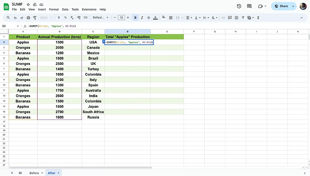
Choose a cell to type the formula

Type “=SUMIF( “ into the selected cell. Then, specify the range of cells you want to evaluate. For example, “=SUMIF(A2:A10, "criteria," B2:B10)”.

4. Step

After selecting the range, enter the criteria that the cells will meet. It can be a specific value or text string like  “Apples, or even conditions like “>10”.

Type the formula and press Enter

Finally, the range of cells is defined to sum up the criteria already met. For instance, “=SUMIF(A2:10, “Apples”, B2:10) sum the values in B2, where cells in A2 meet the criteria “Apples”

💡You can use wildcard characters like “ * ” and “ ? ” in your criteria to match various text patterns, making your SUMIF function more flexible and powerful.

Following these steps, you can use the SUMIF function in Google Sheets to sum the values you want it to calculate.

Frequently asked questions about the SUMIF formula

The SUMIF formula can be a bit tricky, and many users have questions about how to use it properly. Here are some of the most frequently asked questions and answers to help you understand better. Let’s check out what they can be.

Final words

In this guide, we learned how to use the SUMIF function in Google Sheets and the most common questions. We covered the formula, when to use it, and how to apply it step-by-step. With this knowledge, you can now sum values based on specific criteria, making your data analysis faster and more efficient.

For more guides on Google Sheets formulas and functions, follow us. You can find detailed tutorials on other powerful tools like the XLOOKUP function, the UNIQUE function, and the percentile function. Stay tuned for more tips and tricks on mastering Google Sheets and making your data work for you!