How to use the JOIN function in Google Sheets (Detailed steps)

Summarize with
When working with Google Sheets, there are times when you need to combine information from multiple cells into one. Whether you're organizing data, creating lists, or formatting text, merging content can save time and make your sheet easier to read. That’s where the JOIN function helps, allowing you to join multiple pieces of text into one cell easily.
This guide will teach you how to use the JOIN function effectively. We are going to show you how to write the formula, select a separator, and handle both filled and empty cells. By the end, you'll know how to apply the function to join multiple cells and improve the layout of your spreadsheet.
What is the JOIN function?
The JOIN function in Google Sheets lets you join text from different cells into one.
You can choose a separator to connect the words, like a space or comma. It’s a simple way to use the formula in Google Sheets to combine text, making your data look more organized. This is similar to the textjoin Google Sheets function but is more flexible with different separators.
5 reasons to use the JOIN function
The JOIN function is a powerful tool that simplifies data management in Google Sheets. It allows you to combine text from multiple cells into one, making your data clearer and easier to work with. Here are some reasons why you should use it:
🎯 You can merge data from different cells or columns into a single cell.
🎯 It is possible to customize how text is joined by using separators like spaces or commas.
🎯 You can simplify data formatting, especially when working with lists or larger datasets.
🎯 It allows you to handle empty cells without causing errors in your formula.
🎯 You can easily organize mixed data types into one cell for a cleaner look.
How to use the JOIN function (easiest steps)
Now that we’ve covered what the JOIN function is and why it's useful, let’s dive into how to use it. With just a few simple steps, you can combine text from different cells and make your data more organized and readable. You can easily follow along and apply these steps to your own data.
1. Log into your Google account
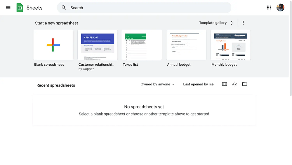
Open your Google Sheets account
Start by logging into your Google account and opening Google Sheets. If you don’t have an existing sheet, create a new one and paste it into the example data, or open a document you’re already working on.
2. Select the range of cells to join
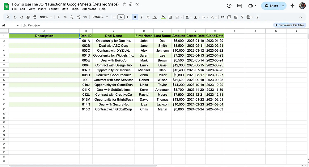
Choose the range of cells
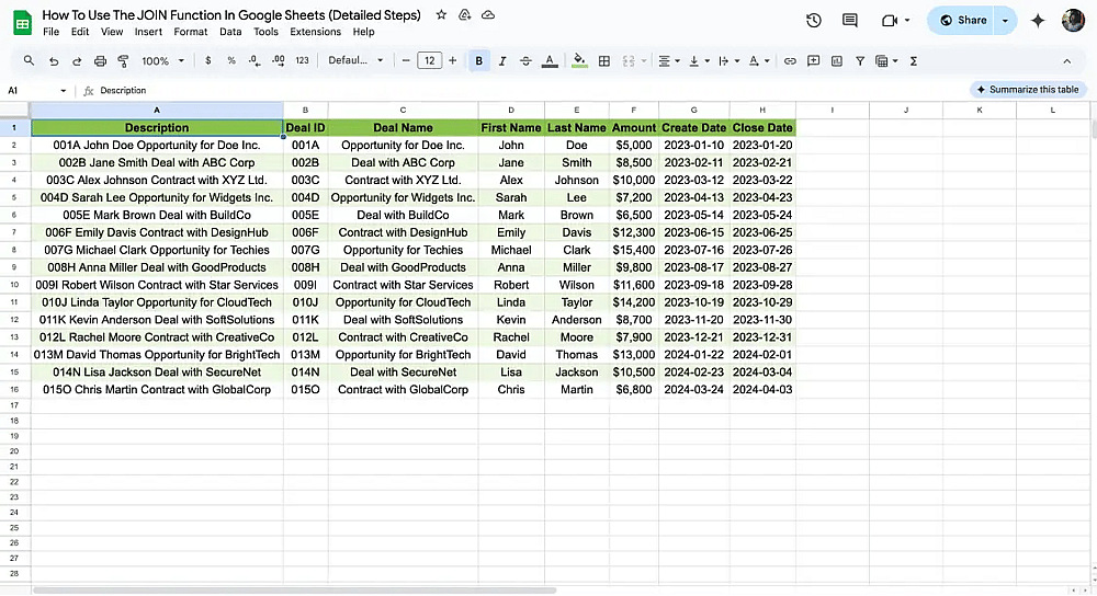
Identify the range of cells you want to combine. For instance, if we are going to join the “Deal ID,” "First Name", "Last Name", and “Deal Name” columns from our table, we need to select cells from these three columns.
3. Enter the formula
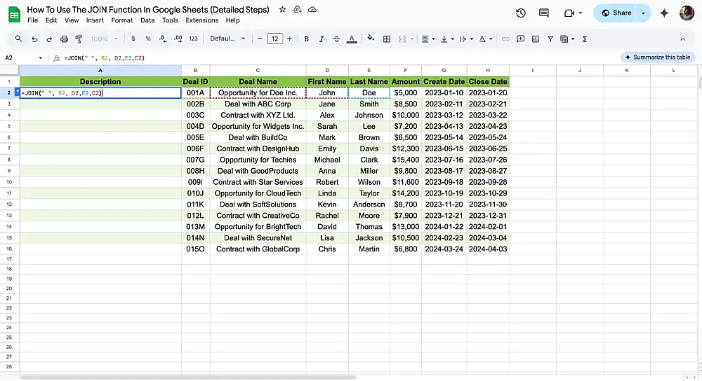
Type the formula
In a new cell (A2 for our example), enter the formula =JOIN(" ", B2,D2, C2,E2). The " " space in the formula acts as the separator between the text in the two cells. The cell reference for the Deal ID is B2, the first name is D2, the last name is E2, and the Deal name is C2.
4. Apply it to other raws
Drag the bottom corner to apply more cells
Press Enter, and the combined text will appear. To apply this formula to the entire column, use one of the most popular Google Sheets tips: Drag the bottom-right corner of the filled cell down to copy the formula to other rows.
Frequently asked questions about the JOIN function
The JOIN function can raise many questions, especially if you are new to Google Sheets formulas or working with large datasets. Below, we answer some common questions to help you better understand how and when to use this useful function.
Google Sheets query can join multiple columns by using the JOIN function within the query formula. This allows you to combine text from different columns while still using query conditions to filter your data. For example, you can join first and last names into a single column while performing a query to display specific rows.
Joining two cells in Google Sheets is easy with the JOIN function. Just type =JOIN(" ", A1, B1) in a new cell. The " " part adds a space between the two cells, but you can switch it to a comma, dash, or anything else you prefer. This way, you can combine the text from both cells into one smoothly.
The TEXTJOIN function in Google Sheets combines text from multiple cells with a specified delimiter, like a comma or space. It can also ignore empty cells, making it more flexible than JOIN. The formula is =TEXTJOIN(", ", TRUE, A1:A5) to merge text while skipping blank cells.
To split text in Google Sheets, you can use the SPLIT function. For example, if you have a cell with text like "John, Doe" and you want to split it into two separate cells, you can use =SPLIT(A1, ", "). This will break the text at the comma and place the separated parts into different cells.
No, it’s not possible to format part of the text as bold or italic directly using the JOIN function in Google Sheets. The function only merges text without any formatting.
Yes, you can use the JOIN function to combine both numbers and text in Google Sheets. For example, =JOIN(" - ", A1, B1) will join the number in A1 and the text in B1, with a dash as a separator. Google Sheets will automatically convert numbers into text when using this function.
Conclusion
We’ve covered everything you need to know about the JOIN function in Google Sheets, from combining text to skipping empty cells. It’s a handy tool for keeping your data organized, whether merging names, IDs, or any other info. Plus, it makes your spreadsheet look way cleaner and easier to manage.
Functions like JOIN are game-changers for saving time and getting your data in shape, especially when juggling a lot of information. If you want more tips and tricks for Google Sheets, don’t hesitate to check out our other guides.
Contributors
forms.app, your free form builder
- Unlimited responses
- Unlimited questions
- Unlimited team members