Google Sheets offers a wide range of functionalities to streamline tasks and improve productivity. Among these features, the ability to wrap text is particularly useful. This function allows users to keep all the content visible in a cell without extending its width. It effectively manages data, preventing text overflow and keeping the sheet neat.
In this guide, we will explore how to use the wrap text feature in Google Sheets and provide a detailed walkthrough. We will cover essential steps like selecting cells, applying the wrap text option, and using keyboard shortcuts to speed up the process. By the end of this article, you will have a clear understanding of the wrap text functionality in Google Sheets.
How to wrap text in Google Sheets
Wrapping text in Google Sheets helps you see all your data in each cell without changing column widths. This guide shows how to use wrap text in Google Sheets. It makes your sheets look neat and organized. You will learn to keep text inside cells, making work easier. Here are the steps for wrapping text in Google Sheets:
1. Step

Google Sheets dashboard
The first step is for text wrapping: sign in to your Google account. Then, open Google Sheets from Google Drive. You can start a new sheet or open an existing one.
2. Step

Choose your data
After opening your sheet, pick the cell or cells where you want to wrap the text. Look for the text wrapping icon in the toolbar. It’s in the format menu. This icon helps you manage how text fits in a cell.
3. Step
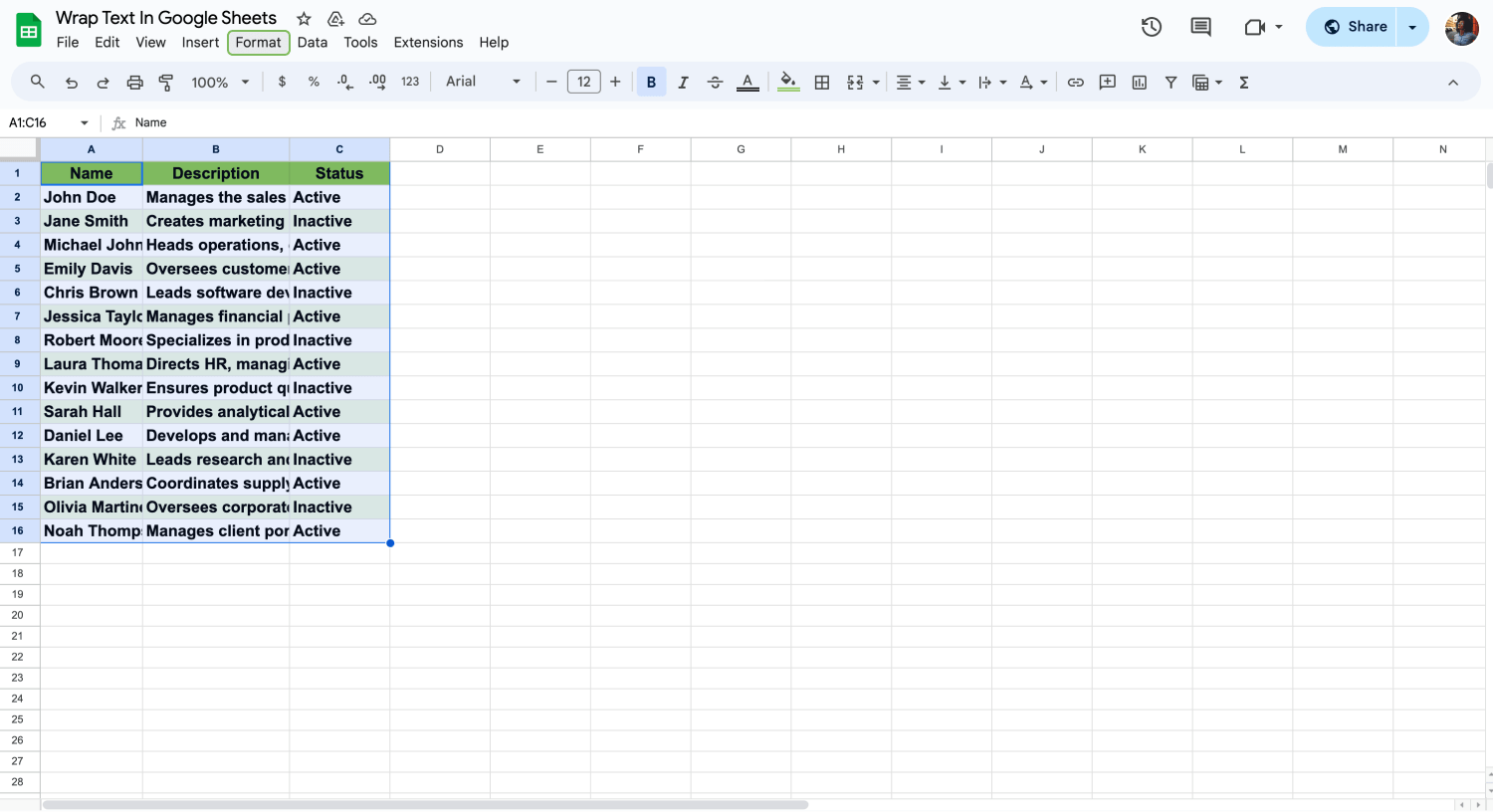
Click “Format”
Go to the 'Format' menu at the top. Here, you will see text-wrapping options. Click on it. This menu lets you control text in cells. It’s where you can wrap the text.
4. Step
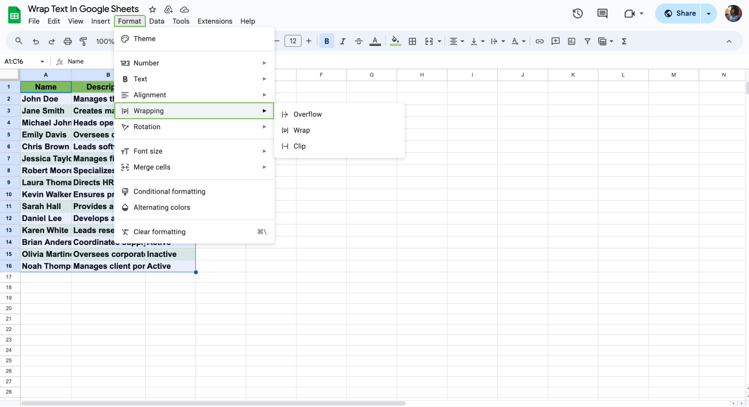
Choose “Wrapping”
In the text wrapping options, select 'wrap'. This makes the text stay inside the cell. It will not overflow. This way, text breaks into lines to fit the cell size.
- Wrap Text: Automatically moves text to a new line within the same cell if it exceeds the cell's width.
- Overflow: Allows text to spill over into adjacent cells if those cells are empty.
- Clip: Cuts off the text that exceeds the cell's width, showing only the part that fits.
5. Step
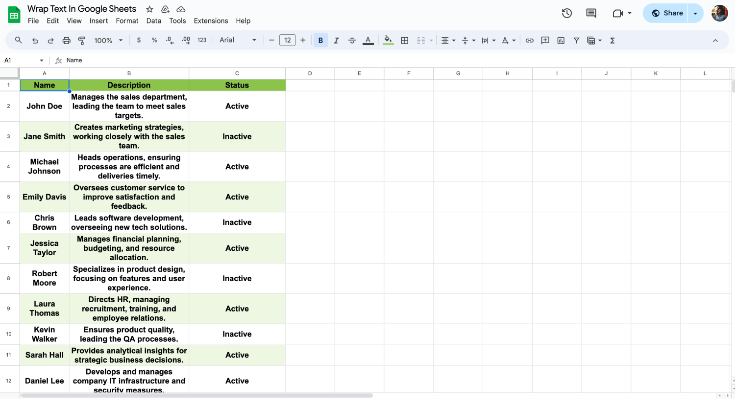
Wrap your text
Once you select 'wrap' from the text wrapping options, check your cell. The text should now fit neatly inside the cell, making your sheet easier to read and more organized.
💡After wrapping your text in Google Sheets, you can align them from the button on the "Format" menu for a cleaner look. You can also play around with columns and line sizes.
Frequently asked questions about wrapping text
Many users have questions about how to use wrapping in Google Sheets effectively. This includes fitting text within cells, adjusting line breaks, and finding shortcuts for quicker formatting. In this section, we'll explore these common inquiries to improve your understanding and use of the Google Sheets app.
To wrap text in a spreadsheet, click on the cell or select multiple cells where you want the text wrapped. Then, go to the "Format" menu, choose "Text wrapping," and select "Wrap." This makes the text fit inside the selected cells, breaking into new lines as needed.
To make all cells fit text in Google Sheets, select the cells or the entire sheet you want to format. Then, use the "Format" menu, choose "Text wrapping," and select "Wrap." This adjusts the cell height to display all text content within the cell boundaries.
In Google Docs, select the text you want to wrap, then go to "Format" in the menu bar, choose "Align & indent," and then "Indentation options." Here, you can adjust text wrapping settings to control how text wraps around elements like images or tables.
Yes, using the how-to wrap text in Google Sheets shortcut makes it quick and easy. Just select the cells you want to format and press Alt + O, followed by W. This shortcut wraps the text in the selected cells efficiently.
Wrap in Google Sheets breaks the text into multiple lines within the cell, while overflow allows the text to extend across the next empty cells. If the adjacent cell is not empty, the text will be cut off at the cell border.
Text wrapping doesn’t directly affect cell width; it only changes how text fits within the existing cell dimensions. To adjust the width, you need to resize the column manually.
To unwrap text, select the cells with wrapped text, go to the "Format" menu, choose "Text wrapping," and then select "Overflow." This will make the text continue in a single line and overflow into adjacent cells if empty.
Text wrapping ensures that all the content in a cell is visible and neatly arranged when printed. Without wrapping, longer text that overflows might not appear fully in the printed document.
In Excel, to wrap text, select the cells you want, go to the "Home" tab, and click "Wrap Text" in the "Alignment" section. This makes the text fit within each cell.
Key points to take away
Learning to wrap text in Google Sheets enhances your data management skills, ensuring that your spreadsheets are clean and organized. This feature is crucial for presenting information clearly, allowing viewers to understand data without the need to continually adjust column sizes.
Google Sheets is a powerful tool for anyone looking to improve their data productivity. By mastering features like text wrapping, you can fully take advantage of Google Sheets's offerings. Stay updated with our guides to discover more tips and tricks for managing and analyzing your data efficiently.
Behçet is a content writer at forms.app. He is a music producer and enjoys blending electronic and acoustic tunes. Behçet has expertise in Google Sheets, survey questions, and online forms.
