In the world of Google Sheets, it is essential to be able to find a specific piece of information quickly. The XLOOKUP function comes into play, especially when dealing with large amounts of data. This tool significantly simplifies the process of searching through data.
The XLOOKUP formula transforms how we interact with data in Google Sheets, departing from traditional lookup formulas. It offers a fast and accurate way to sift through information, boosting efficiency across tasks. In this guide, we'll walk you through the basics of using XLOOKUP in Google Sheets and guide you on how to leverage its power in your data management workflows.
What is the XLOOKUP function in Google Sheets?
The XLOOKUP function in Google Sheets is a powerful tool that searches and retrieves information with precision and flexibility.
It goes beyond the traditional VLOOKUP formula. XLOOKUP allows advanced searches, including match mode argument. If you compare XLOOKUP vs VLOOKUP, you will see a big flexibility difference in usability. An XLOOKUP example demonstrates searching in any direction. Unlikely, VLOOKUP has a vertical limit, especially when it is about direction. You can look for exact matches, approximate matches, or wildcard matches.
When to use the XLOOKUP function
XLOOKUP not only finds data but also smartly goes through it, making searches in Google Sheets faster and more precise. If you're unsure of what to look for, adding a question mark helps find close matches. This flexibility works when you work with data on lists sorted up or down, fitting perfectly into your workflow.
⏰It's invaluable for working with datasets that are neatly organized.
⏰It excels when dealing with values sorted in ascending order.
⏰It's also handy for data sorted in the opposite or descending direction.
💡For more data tips, you can check out the UNIQUE function in Google Sheets to easily clean up your data.
What's the difference between VLOOKUP and XLOOKUP?
Google Sheets formulas are lifesavers. There are various ways to ease your workflow. VLOOKUP and XLOOKUP are only two of the important formulas. They bring better flexibility and ease of use to spreadsheets. However, XLOOKUP goes beyond VLOOKUP. It allows searches in any direction. XLOOKUP also offers more advanced options. This makes finding data in Google Sheets simpler and more efficient. Here are some differences:
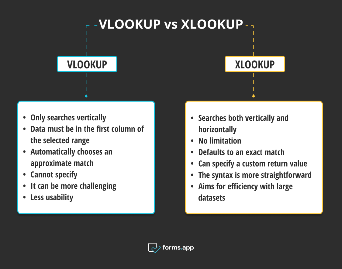
Differences between VLOOKUP and XLOOKUP
🎯Search direction: VLOOKUP can only search vertically (down columns), starting from the leftmost column. XLOOKUP can search both vertically and horizontally (across rows), offering greater versatility.
🎯Lookup column limitation: With VLOOKUP, the lookup value must be in the first column of the selected range, and the return value must be in a column to the right. XLOOKUP doesn't have this limitation; you can return values from any column, regardless of the lookup column's position.
🎯Default match type: If you don't specify the last argument, VLOOKUP automatically chooses an approximate match. This can cause errors if you haven't sorted the range correctly. XLOOKUP defaults to an exact match, reducing the chance of errors.
🎯Return value for not found: You can specify a custom return value in XLOOKUP if it doesn't find the lookup value. This feature is not available in VLOOKUP without being wrapped up in an error-handling function.
🎯Simplicity and readability: XLOOKUP's syntax is more straightforward, making formulas easier to read and write. With VLOOKUP, understanding and maintaining complex formulas can be more challenging, especially for new users.
🎯Performance: XLOOKUP aims for efficiency with large datasets, avoiding a search through the entire column or row after finding a match.
How to use the XLOOKUP function in Google Sheets
Using the XLOOKUP function in Google Sheets is straightforward once you understand the basics. Thanks to the formula, you specify the exact piece of data XLOOKUP should be found in your Google Sheet. Here are some steps for you to use the function:
Step 1
Begin by opening the Google Sheets document that contains the data you need to analyze.
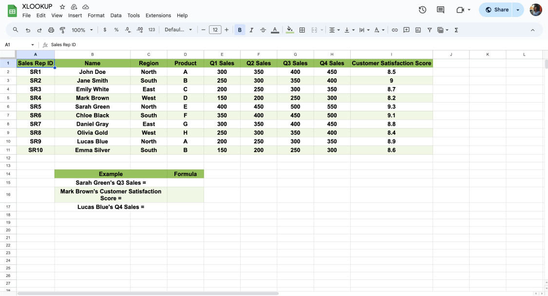
Open your sheet
Step 2
Choose a clear cell to start writing your function. Make sure the cell is empty to avoid any errors.
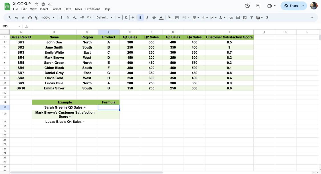
Click cell to type the formula
Step 3
Becoming familiar with the XLOOKUP function's basic formula plays a crucial role. The structure =XLOOKUP("Sarah Green", B2:B11, F2:F11) includes:
- “Sarah Green” : lookup_value: the target of your search.
- “B2:B11” : lookup_range: This is where your search unfolds.
- “F2:F11” : return_range: It is the source of your answer.
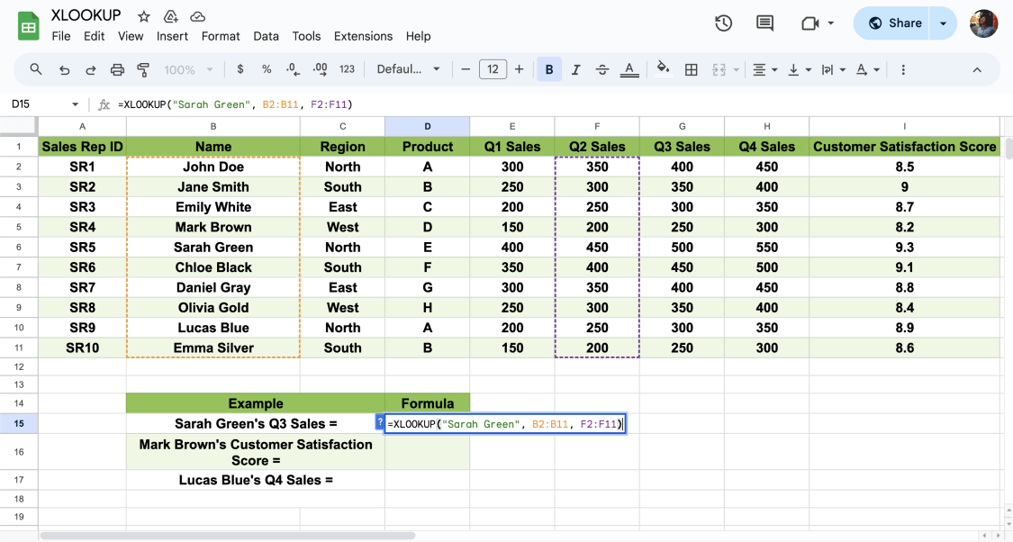
Type the formula
Optional elements add depth to your search:
- If_not_found: It offers an alternative when searches fall short.
- Match_mode: It fine-tunes the precision of your match.
- Search_mode: It guides the direction of your search.
Step 4
Now comes the exciting part—finding the information we need! With our criteria set, we input them into the XLOOKUP function. Once you're ready, type in your formula. Hit Enter, and watch as the sought-after data reveals itself on your spreadsheet.
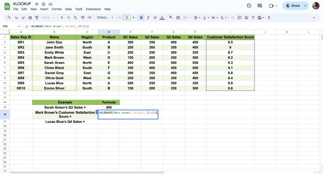
Click enter to see the result
Step 5
After successfully finding the data with XLOOKUP, it's time to review the results. Consider how you can utilize the information obtained in your analysis or reporting. This step enhances your work, allowing you to navigate complex datasets in Google Sheets more efficiently.
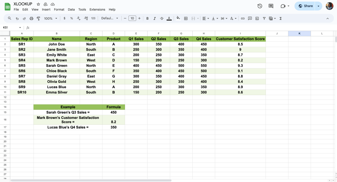
Analyze the final result
Frequently asked questions about the XLOOKUP function
Diving into XLOOKUP in Google Sheets can bring up lots of questions for beginners. This guide is easy to follow, whether you're new to it or already know a bit about the XLOOKUP function. This title aims to enhance user proficiency with the XLOOKUP function, making data management significantly more efficient.
XLOOKUP searches for a specific value in a range or array and returns a corresponding value from another range or array. Using the XLOOKUP function allows both vertical and horizontal lookups.
XLOOKUP combines the capabilities of both VLOOKUP and HLOOKUP, offering more flexibility. It can look up data in any direction and find related items without the restrictions of older functions.
Yes, XLOOKUP can handle two criteria when you pair it with functions like FILTER or use it in an array formula. This allows you to perform more complex searches that match both conditions you specify.
Yes, XLOOKUP can work with arrays, allowing it to return multiple values at once.
Yes, XLOOKUP supports wildcard characters like the asterisk (*) and question mark (?), making it possible to search for partial matches.
XLOOKUP is available in Excel for Microsoft 365 and Excel 2019. For Google Sheets users, XLOOKUP is readily available and does not depend on the software version.
- Identify your lookup value: This is the value you want to find in your spreadsheet.
- Determine your lookup array: This is the range of cells where Excel will search for the lookup value.
- Select your return array: This is the range of cells from which Excel will return the value corresponding to the lookup value.
- Write the XLOOKUP formula: Click on the cell where you want the result to appear, and type in the XLOOKUP formula using the syntax =XLOOKUP(lookup_value, lookup_array, return_array). Optionally, you can include additional arguments for if_not_found, match_mode, and search_mode to customize the function's behavior.
- Press Enter: After entering the formula, press Enter. Excel will process the function and display the matching return value in the selected cell.
XLOOKUP lets you set a custom return value for when it doesn't find the search key, making it easier to handle errors.
Unlike the VLOOKUP function, XLOOKUP can easily return values from columns to the left of the search column, as it does not restrict the return range's position.
Based on the search mode you specify, XLOOKUP searches for and returns the first match, as its design primarily focuses on finding a single match.
To look up data using multiple criteria in Excel or Google Sheets, you have a few options. Excel users can use the INDEX and MATCH functions together for complex searches. Google Sheets offers the FILTER function, which is simpler and can easily handle multiple conditions. This lets you quickly find the data you need by setting more than one rule for your search.
Last words
Exploring XLOOKUP in Google Sheets changes the game in data handling. It highlights optional arguments and the lookup value table array and moves us past the old VLOOKUP methods. These features are essential for anyone looking to sharpen their data analysis and precision.
This guide introduced XLOOKUP's advanced features and showed how to use them effectively.
Using these XLOOKUP strategies can make your projects more efficient and accurate. Optional arguments and the lookup value table array take your Google Sheets skills to the next level. These methods open up new possibilities for managing data. With these techniques, you can tap into Google Sheets' full potential for better data analysis and planning!
Behçet is a content writer at forms.app. He is a music producer and enjoys blending electronic and acoustic tunes. Behçet has expertise in Google Sheets, survey questions, and online forms.
