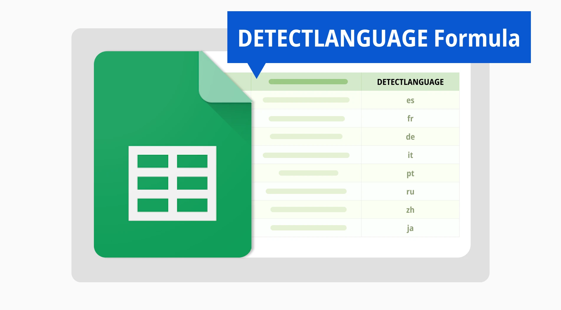
Understanding something is the first step in decoding or learning it, and language is the first thing that we have to know if we want to understand something. Knowing and understanding a language is always important in every business sector, and Google Sheets is no exception. That is why it is necessary to learn how the DETECTLANGUAGE function works.
In this article, we will examine the DETECTLANGUAGE function and how to use the language detector function in Google Sheets. We will also look at some of the frequently asked questions about the DETECTLANGUAGE formula to better understand the details of this feature.
What is the DETECTLANGUAGE function?

The DETECTLANGUAGE function detects the language of a text in a specific cell range.
Arguably one of the easiest functions to learn among all of the Google Sheets formulas, this language detection model offers great help for text-heavy folders. One of the best features of this function is that it can detect the language of a text in a specific cell or multiple cells in a certain cell range.
How to use the DETECTLANGUAGE function in Google Sheets
As it is one of the easiest functions to learn and use, the DETECTLANGUAGE function does not need any extensive tips and tricks to implement. However, there are still things to keep in mind, such as the function not giving the result that is needed all the time due to similarities in languages.
1. Open your Google Sheets folder and locate the cell(s)
The first step that you must do to use the DETECTLANGUAGE function is to open your Google Sheets folder and locate the cell or cells that you would like to use the function on. One important thing to keep in mind is to make sure that you correctly locate the individual cell or the cell range that you would like to use.
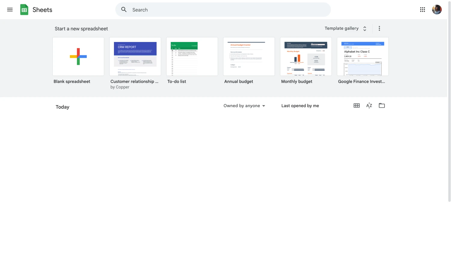
Choose or start a new sheet

💡As the DETECTLANGUAGE function can only work with text values, it is important to select the cells that have texts in them. Otherwise, you will be unable to get the results that you want.
2. Select a blank cell and type in your function
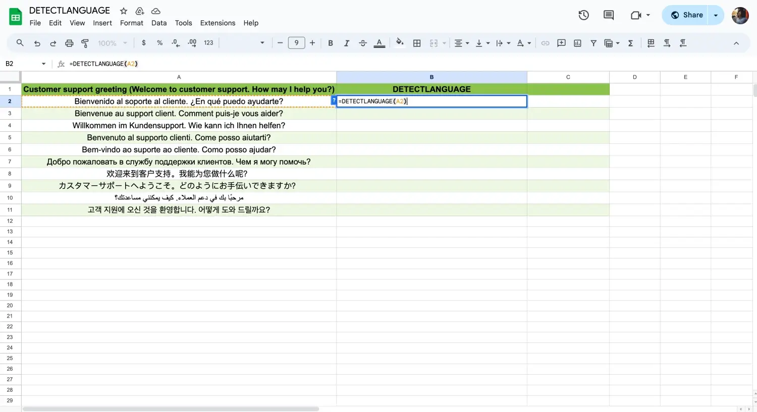
Type the formula
After you locate the individual cell or the cell range that you would like to use, the second step in using the language identification feature is clicking on a blank cell and typing =DETECTLANGUAGE. Afterward, you will have to type which cell or cell range you would like to use in parentheses. Google Sheets will give you the results from the language identifier in real time.
3. Press Enter
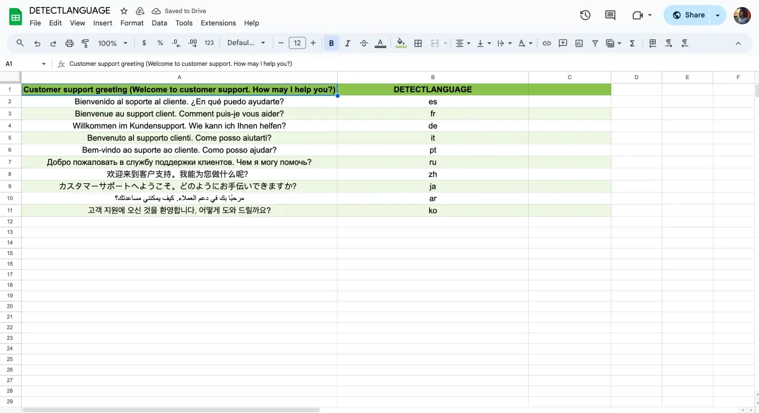
Press enter
After you type in your function, all that is left to do is press enter and let Google Sheets calculate the results in real time. Make sure to check the cell range and the data that you have typed several times to look for any errors, and keep in mind that the DETECTLANGUAGE function does not always give the correct result. So be prepared to do some post-editing.
Frequently asked questions about the DETECTLANGUAGE formula
Now that you have learned how to use the DETECTLANGUAGE function to identify a language, it is time to dive into the tips and tricks with the help of answering some of the frequently asked questions about the DETECTLANGUAGE formula.
Como o nome sugere, a fórmula GOOGLETRANSLATE ajuda a traduzir textos dentro de uma célula ou intervalo de células usando o Google Translate. Há várias coisas importantes a ter em mente ao usar esta fórmula. Como o Google Translate é um aplicativo de aprendizado de máquina baseado em idioma, assim como todos os outros aplicativos de tradução, é importante usá-lo com frequência para obter melhores resultados.
A fórmula básica de tradução que você pode usar para o Google Sheets é a fórmula GOOGLETRANSLATE. Esta fórmula ajuda a traduzir mais de 100 idiomas e funciona em idiomas escritos e falados. Esta função não o obriga a depender de aplicativos de terceiros; é ótimo para empresas internacionais.
Você também pode usar a função de detecção de idioma no Excel, pois é um recurso que o Excel também oferece. No entanto, você só pode detectar um idioma no Excel, pois não há função que entenda idiomas e os traduza para um idioma desejado. Embora haja um recurso de tradução no Excel, você teria que baixar um complemento para que ele funcione em células.
O processo de verificar idiomas em uma célula individual ou em um intervalo de células é o mesmo que no Google Sheets. Você só precisa localizar as células que deseja usar, clicar em uma célula em branco e digitar a função de detecção de idioma. Em seguida, basta digitar o intervalo de células que você deseja usar entre parênteses e obter os resultados.
Key points to take away
In summary, the DETECTLANGUAGE function can be quite useful for international businesses with text-heavy documents. It is a great way to identify and organize certain text groups within a folder. However, some post-editing may be necessary as this feature is not perfect due to similarities between languages.
In this article, we have looked at what the DETECTLANGUAGE function is, and how to use the DETECTLANGUAGE function in Google Sheets. We have also examined several of the frequently asked questions about the DETECTLANGUAGE formula for Google Sheets and Excel. It is now time for you to apply your new skills and use it as a stepping stone for your success.
Yakup is a content writer at forms.app. He is also a skilled translator. His hobbies include reading, learning about different languages, and different branches of sports. Yakup's expertise lies in translation, NoCode tools, and Google Forms.


 3 min ler