Google Sheets has many functions that allow you to work with and look at your data in useful ways. Functions like WEEKDAY make it easier to handle dates. The functions help you see patterns, plan your schedule, and understand when things happen simply. Even if you're new to using functions, the WEEKDAY function can make your spreadsheet more powerful and easier to use.
In the following parts, we'll focus on the WEEKDAY function. We'll answer some common questions and show you step-by-step how to use it. You'll see how it can be handy through practical examples that demonstrate its everyday utility.
What is the WEEKDAY function?

The WEEKDAY function is a formula in Google Sheets that returns the day of the week as a number for any given date, where 1 represents Sunday and 7 represents Saturday.
This function is particularly useful for organizing and analyzing data based on days of the week, helping users to schedule tasks and track weekly cycles efficiently.
How to use the WEEKDAY function in Google Sheets
Using the WEEKDAY function in Google Sheets allows you to manage and analyze dates within your data effectively. This simple yet powerful function can help streamline project timelines, track events, and organize weekly tasks by identifying days of the week for specific dates. Let’s walk through the steps to use this function effectively.
1. Open Google Sheets
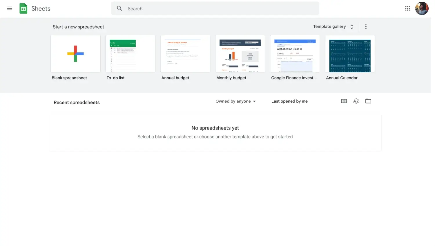
Log into your Google account
Start by signing into your Google account and opening a spreadsheet.
2. Select a cell
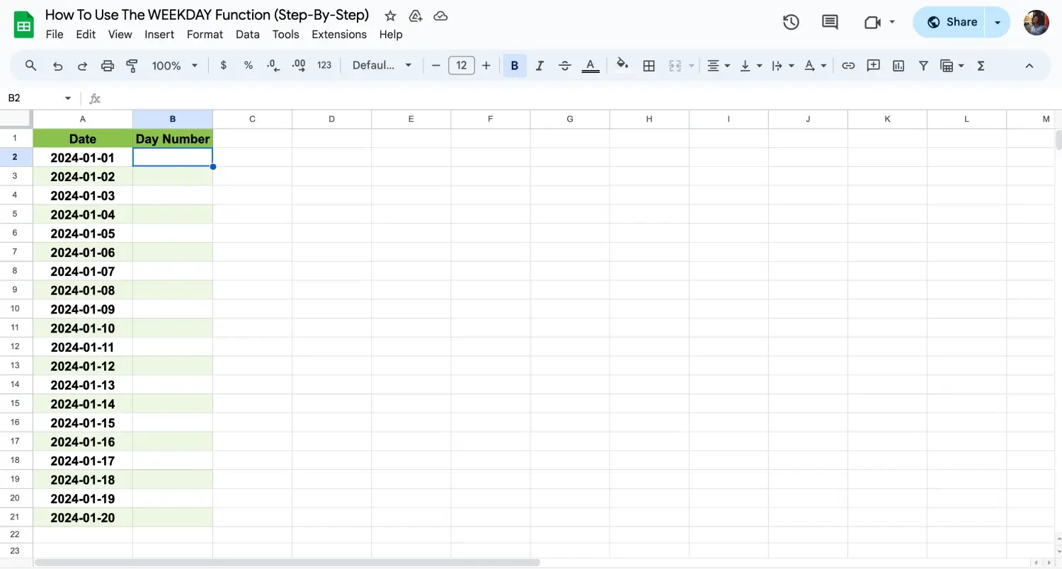
Choose a cell to apply the formula
Click on the cell where you want to use the WEEKDAY function. The result will appear here.
3. Type the function
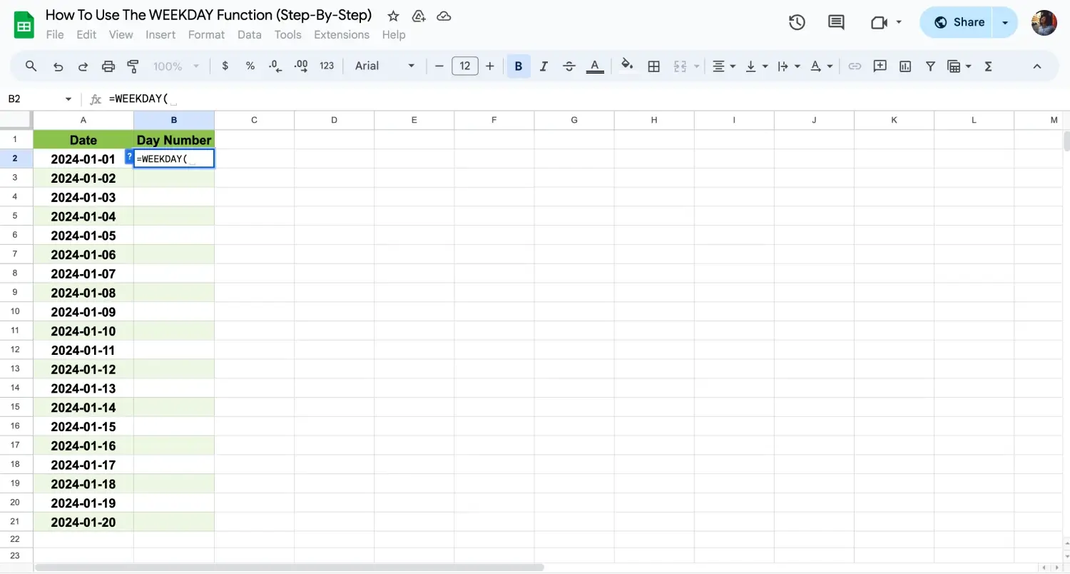
Type the formula
Enter “=WEEKDAY( “ into the cell. Then, provide the date you want to analyze.
4. Specify the date
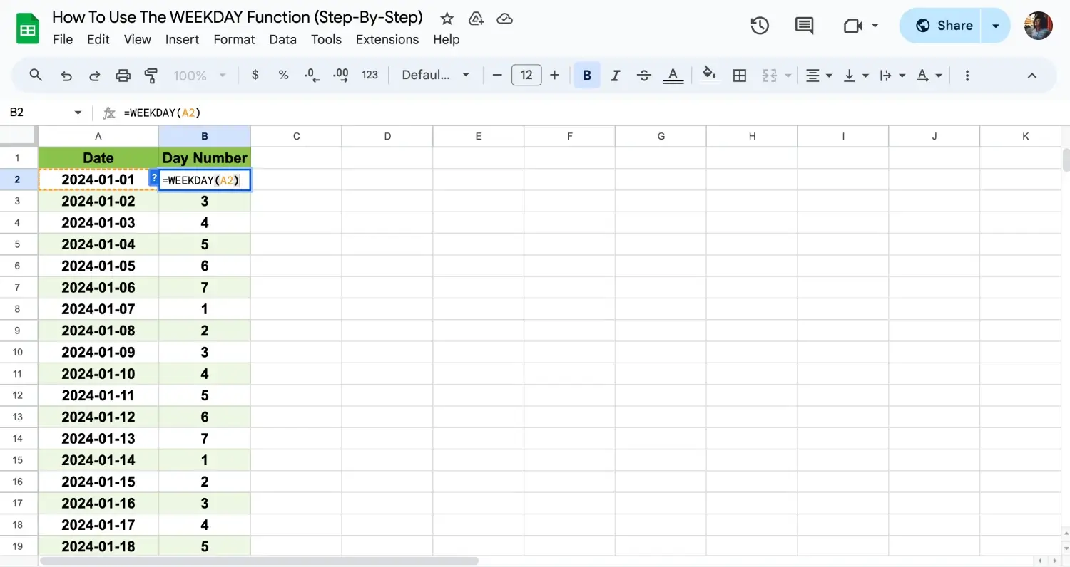
Apply the formula to the other cells
Add the reference for the cell containing the date or type the date directly inside quotation marks. For example, “=WEEKDAY(A2)” or “=WEEKDAY("2023-10-01")”.
5. Press Enter
Close the function with a parenthesis “)” and press Enter. The cell will now show the day number of the week for your specified date.
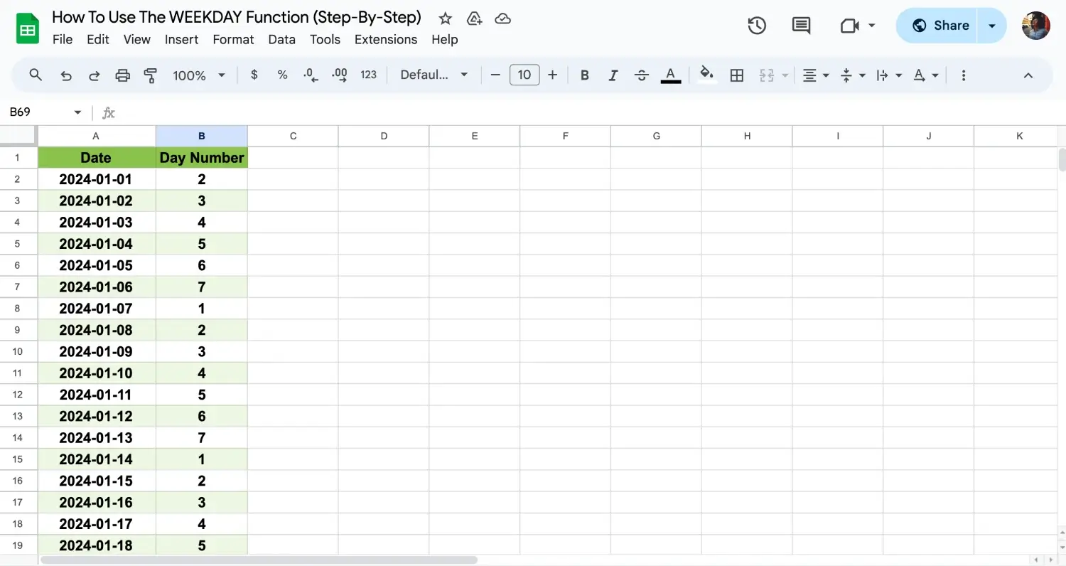
Click Enter
By following these steps, you'll be able to use the WEEKDAY function in Google Sheets to organize your data by the days of the week.
WEEKDAY vs. LOOKUP
Understanding the differences between the WEEKDAY and LOOKUP functions in Google Sheets can help you choose the right tool for your data tasks. While both functions are useful for managing data, they serve different purposes and operate in distinct ways.
Here’s a quick comparison of the WEEKDAY and LOOKUP functions:
🎯Purpose: WEEKDAY is used to find the day of the week for a given date and returns a numerical value representing each day. LOOKUP, on the other hand, searches for a value in a row or column and returns a corresponding value from another row or column in the same range.
⚙️Usage: WEEKDAY is ideal for date-related calculations, helping to organize schedules or analyze trends based on days of the week. LOOKUP is more versatile for searching within data, such as finding a price based on a product ID or matching employee names with their IDs.
🕹️Input requirements: The WEEKDAY function requires a date input and optionally allows you to specify the type of numbering you want for days of the week. LOOKUP requires two arguments: the value to search for and the range to search within.
📤Output: The output of WEEKDAY is a simple integer (1-7) indicating the day of the week. LOOKUP’s output is the matched data from the search range, which could be any type of data, such as text, numbers, or dates.
Understanding these differences will enable you to use each function more effectively in your Google Sheets projects.

💡Tip: You can also use the XLOOKUP function for flexible searches and the UNIQUE function to find distinct values, enhancing your Google Sheets analysis.
Frequently asked questions about the WEEKDAY function
The WEEKDAY function is a handy tool in Google Sheets for dealing with date data, but it can raise questions, especially for new users. This section aims to clear up some of the most common queries related to the WEEKDAY function and similar date-related functions.
Um Wochentage in Google Sheets aufzulisten, geben Sie ein Startdatum in Zelle A1 ein. In A2 geben Sie `=A1+1` ein und ziehen es nach unten, um eine Sequenz von Daten zu erstellen. Verwenden Sie dann `=TEXT(A1, "dddd")` in Zelle B1 und ziehen Sie es nach unten, um diese Daten in Wochentagsnamen umzuwandeln und jeden Tag neben seinem Datum anzuzeigen.
Die WORKDAY-Funktion hilft Ihnen, ein Datum in der Zukunft oder Vergangenheit basierend auf einer angegebenen Anzahl von Arbeitstagen zu berechnen. Zum Beispiel berechnet `=WORKDAY(A1, 10)` das Datum, das 10 Arbeitstage nach dem Datum in Zelle A1 liegt, unter Ausschluss von Wochenenden und optional auch Feiertagen.
Die DAYS-Funktion berechnet die Anzahl der Tage zwischen zwei Daten. Geben Sie einfach das Startdatum und das Enddatum als Parameter ein, wie `=TAGE("2023-12-31", "2023-01-01")`, das die Anzahl der Tage vom 1. Januar bis zum 31. Dezember 2023 zurückgibt.
Die WEEKDAY-Formel in Excel funktioniert ähnlich wie in Google Sheets. Sie gibt den Wochentag zurück, der einem Datum entspricht. Zum Beispiel gibt `=WEEKDAY("2023-10-01", 1)` den numerischen Wochentag für den 1. Oktober 2023 zurück, wobei die Woche am Sonntag beginnt.
Final words
Throughout this guide, we've explored how to utilize the WEEKDAY function in Google Sheets, offering a deeper understanding of how to manage and analyze date-related data efficiently. We've covered practical applications, from listing weekdays to calculating workdays, which can significantly enhance your ability to plan and organize within your spreadsheets.
For more insights like these and to learn additional Google Sheets formulas, continue following our updates. Discover how to add a date picker in Google Sheets and many other useful tricks that will elevate your data handling skills to the next level. Stay tuned for more helpful tips and guides that make navigating Google Sheets a breeze.
Behçet is a content writer at forms.app. He is a music producer and enjoys blending electronic and acoustic tunes. Behçet has expertise in Google Sheets, survey questions, and online forms.


 4 min lesen