
Using Google Sheets to analyze and organize your data will take you far. The SORT feature in the Google Sheets application is one of the most important features you should make use of. Using the SORT function while organizing your data in Google Sheets will make your data more meaningful and prevent confusion.
Using the Google Sheets SORT function in multiple columns when analyzing data will make your work easier and allow you to make faster comparisons. In this guide, we will explain the SORT feature and how to use it. With this guide we have prepared for you, you will improve your data analysis experience. Let's move on to our informative article without wasting any more time.
What is the SORT function in Google Sheets?

The SORT function in Google Sheets sorts the rows in a given array or range according to the data in one or more columns.
With the SORT function, you can SORT your data in ascending and descending order and analyze it effectively. In this way, you can make your job easier when analyzing data and increase the productivity you get. You can access the data you want practically thanks to the ability to SORT your data according to multiple criteria automatically.
How to use the SORT formula in Google Sheets (step-by-step)
Understanding how to use the SORT formula and using it in your work will make your tasks easier. In this section, we will explain the use of the SORT formula step by step, and you will find answers to all your questions. Here are the steps to teach you the SORT formula:
Step 1. Open the Google Sheets file where you want to analyze the data and select a blank cell without any data. In this blank cell, you will type your SORT function.
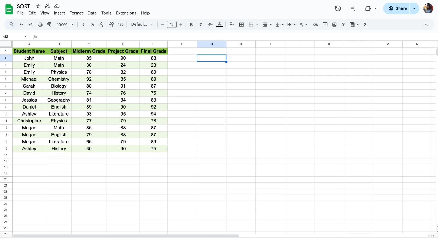
Choose a cell to type the formula
Step 2. Before using the SORT function, you must learn its structure and insert the necessary data. The formula is =SORT(RANGE; SORT COLUMN; TRUE OR FALSE). You can optionally add a specific column and its condition to the formula.
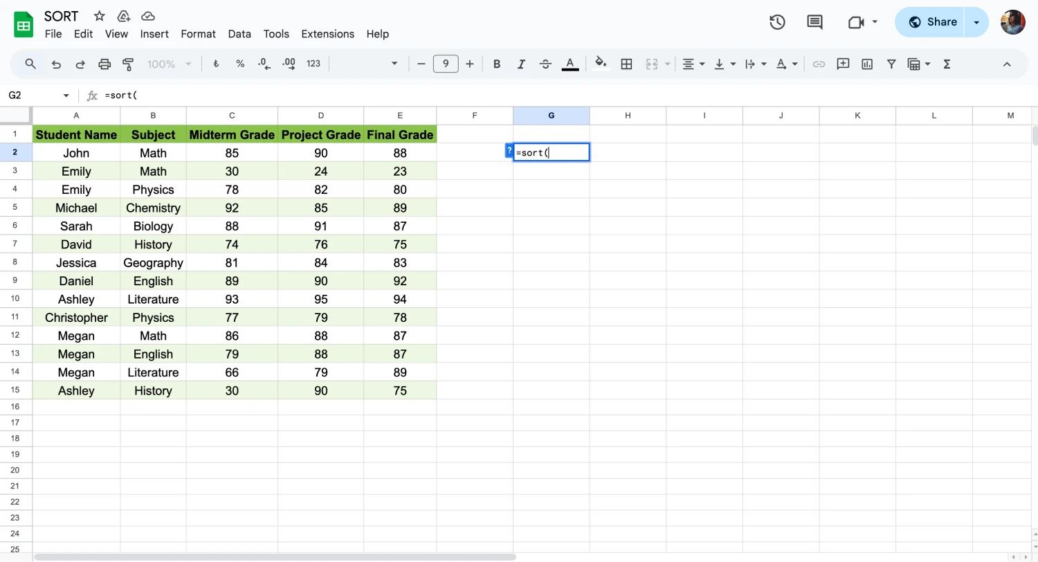
Start typing the formula
- TRUE means that this formula will sort the data in ascending order.
- FALSE means that the data will be sorted in descending order.
Step 3. Now, you should type the SORT formula into your selected blank cell. For example, you can write a formula like =SORT(A2:E15;C2:C15;FALSE;D2:D15;TRUE). When determining the data range, you should select accordingly if your data has a header row.
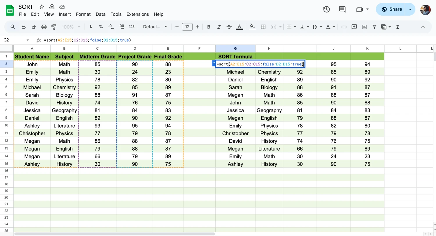
Check the formula
- In this formula, A2:E15 represents the range of data you will sort.
- C2:C15 indicates the column with the first sort criteria.
- FALSE indicates that column C2:15 will be sorted in descending order.
- D2:D15 indicates the column with the second sort criteria.
- TRUE indicates that the data in column D2:D15 will be sorted in ascending order.
Step 4. Click the Enter key and see the data sorted in the selected column. After sorting the data set, you can quickly analyze them and manage big data.
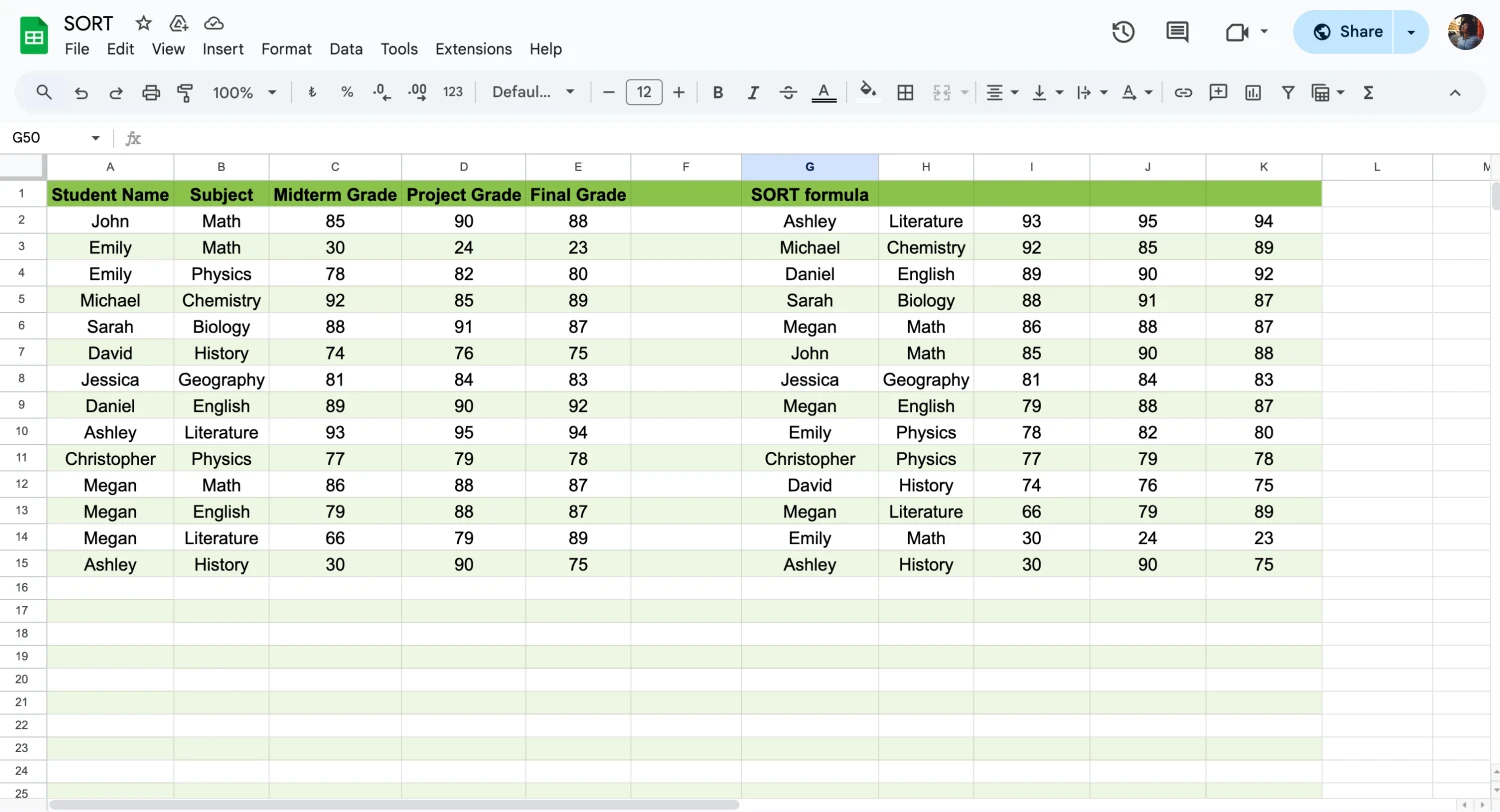
Click Enter and check the result
How to use the SORT and FILTER functions together
Using SORT and FILTER functions together when sorting cells in Google Sheets allows you to achieve efficient results in extensive data management. To learn how to use the FILTER function and its benefits, you can read our article on how to use the filter function in Google Sheets. Now, let's move on to how to use these two functions together:
Step 1. To use SORT and FILTER functions together, create a FILTER formula, as we explained in our previous article. For example, let's look at the formula =FILTER(A2:E15;D2:D15>80).
Step 2. Then, add the SORT formula to the beginning of the formula you created and select the column you want to sort. E.g. =SORT(FILTER(A2:E15;D2:D15>80);5;TRUE). In this formula, 5 refers to the 5th column in the selected range.
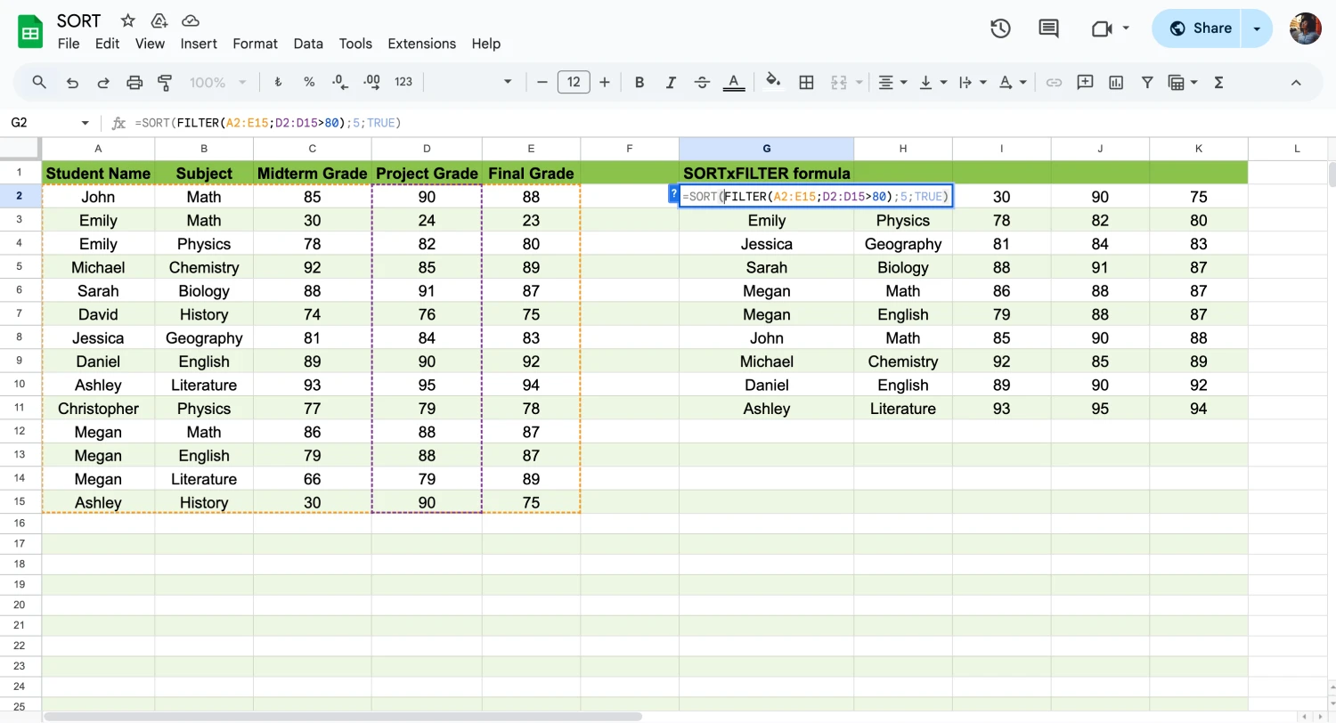
The usage of sort and filter formula
Step 3. Click Enter and start using these two functions to improve your data analysis experience.

💡If you are curious about more useful Google Sheets functions, check out our article about the XLOOKUP function and get ideas.
Frequently asked questions about the SORT function
When you start using the SORT function of Google Sheets, it may seem complicated at first. However, the use of this function is very important for data management. For this reason, let's move on to the section where we answer frequently asked questions so that you can learn the subject better:
Evet. Sağ tıklayıp Daha Fazla Hücre İşlemi Görüntüle'yi seçebilir, ardından Sıralama Aralığı’nı seçebilirsiniz. Verilerinizin bir başlık satırı olup olmadığına göre seçim yapın. Ardından A'dan Z'ye veya tersine göre verilerinizi sıralayabilirsiniz. Eğer birden fazla sütunda sıralama yapmak istiyorsanız Başka Bir Sıralama Sütunu seçeneğini seçebilirsiniz.
Formülünüzü kullanarak sıralamak istediğiniz aralığı belirtin. Ardından, yukarıdaki örnekte olduğu gibi FALSE kodunu girin. Bu şekilde, verileri en yüksekten en düşüğe doğru sıralayabilirsiniz.
Evet. Bu işlevi kullanmak için veri aralığını belirtmeniz, veriye tıklamanız ve Daha Fazla Hücre Eylemi seçeneğini seçmeniz gerekiyor. Ardından sıralama aralığı seçeneğine tıklayabilir ve verilerinizi A'dan Z'ye veya Z'den A'ya sıralayabilirsiniz. Böylece verilerinizi alfabetik sıraya göre dizebilirsiniz.
Google Sheets sorgusunun sayıya göre mi yoksa alfabetik olarak mı sıralanacağını seçebilirsiniz. Verilerinizi sayılara göre sıralarken önce sıralamak istediğiniz sütunu seçmelisiniz. Ardından DOĞRU veya YANLIŞ ekleyerek Google Sheets’te verileri azalan veya artan şeklinde sıralayabilirsiniz.
Wrapping it up
Google Sheets formulas will make it easier for you to collect and analyze data. Thanks to the SORT formula, being able to sort by multiple columns in Google Sheets takes you forward when working with massive data sets. This way, you can quickly access the necessary data and get ahead of your competitors.
Now that you know how to use Google Sheets's SORT function, you are ready to analyze big data sets!
Behçet is a content writer at forms.app. He is a music producer and enjoys blending electronic and acoustic tunes. Behçet has expertise in Google Sheets, survey questions, and online forms.


 3 dakikalık okuma